Climate-Based Daylight Modeling

 Ian Ashdown, P. Eng., FIES, Senior Scientist, SunTracker Technologies Ltd.

Published:  2016/03/26

daylight, n. The light of day.

Apart from having a wonderfully circular definition in most English-language dictionaries, daylight really is just another form of illumination. As such, most people would expect lighting designers to be able to simulate daylight with the same ease that we simulate electric lighting … but ah, I see you blushing.

We have for the past one hundred and fifty years relied on daylight factors to predict the distribution of daylight in architectural spaces. The daylight factor metric is exceedingly simple to calculate, but it is not very useful in understanding how daylight illuminates an interior space. All it really tells us (and our clients) is whether there will be sufficient daylight to read a newspaper indoors on an overcast day. We have, in other words, good reason to blush.

We know better, of course. Given the architectural plans of a building, including both its geographical coordinates and orientation, we know we can use historical weather data to determine the typical distribution of daylight within the building for every hour of every day of the year. We even have a name for this: climate-based daylight modeling (CBDM), an expression introduced a decade ago at a CIBSE lighting conference appropriately called “Engineering the Future” (Mardaljevic 2006).

With CBDM, we can calculate daylight metrics such as spatial Daylight Availability and Annual Sunlight Exposure (IES 2012), Useful Daylight Illuminance (Nabil et al. 2006), Daylight Glare Probability (Wienold et al. 2006), and more.  The first two metrics are important in that they are necessary for earning all three LEED v4 daylighting credit points (USGBC 2013). As consultants to architectural firms, lighting design professionals have an obligation to provide these metrics. Glare metrics take this one step further, offering the ability to identify potential design problems with large expanses of glazing.

Going further still, we can design and validate daylight harvesting systems for energy savings, and address building energy modeling issues involving solar insolation. Most important, we can work with architects during the conceptual design phase to take full advantage of what daylighting has to offer. From a lighting design perspective, CBDM expands the consulting services we can provide.

… and yet we persist in using daylight factors for our lighting design work.

The problem for most lighting designers is that the practice of climate-based daylight modeling is anything but simple. Until recently, the only software capable of performing CBDM calculations has been Lawrence Berkeley National Laboratory’s Radiance … and here I must pause.

Radiance

Radiance is — there are no other words to describe it — an exceedingly powerful, and indeed wonderful, set of software tools for electric lighting and daylighting research. It is not a monolithic program, but rather a set of one hundred or so Unix programs that can be linked together using command-line scripts.

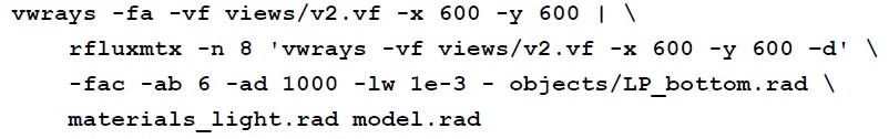
Radiance, however, is first and foremost a research tool. It is reasonable to assume that most architects and engineers will prefer not to learn Unix, with command-line scripts such as:

Fortunately, there are a number of free and commercial architectural-engineering design applications that are available, and which provide graphical user interfaces to the Radiance toolset. Those that support climate-based daylight modeling include DAYSIM and DIVA for Rhino (www.daysim.ning.com).

This article is not, however, about Radiance and its derivatives; it is about climate-based daylight modeling. More particularly, it is about a unique radiosity-based approach to CBDM calculations that does not involve the Radiance daylight calculation engine. It is the culmination of over twelve years of research and development, beginning with the paper “Modeling Daylight for Interior Environments” (Ashdown 2004). The details are disclosed herein for those interested in understanding how it works.

Follow the Light

In order to fully understand the radiosity approach, it is necessary to follow the light from source to receiver. The source is the combination of direct sunlight and diffuse daylight; the receiver is a room or similar naturally illuminated space within a building.

Modeling direct sunlight is straightforward. The solar position in the sky can be readily calculated from the equations presented in Section 7.1.5, Solar Position, of the IESNA Lighting Handbook, Tenth Edition (IES 2011). The solar disk is only 0.5 degrees in apparent width, and so it can be reasonably modeled as an infinitely distant point source that produces a beam of light whose rays are parallel.

Modeling diffuse daylight is more challenging. Some of the extraterrestrial radiation from the sun is scattered by the Earth’s atmosphere, resulting in the hemispherical diffuse light source that is the sky. The sky luminance (colloquially, “brightness”) spatial distribution varies with geographic location, site altitude, time of day, time of year, and weather conditions, including clouds and aerosols such as smoke and airborne dust, and also the dew point temperature.

It is clearly not practical to deterministically model realistic weather conditions, especially partly cloudy weather where the sky luminance distribution may vary on a time scale of minutes. Modeling diffuse daylight therefore requires a simplifying mathematical model, which in turn requires measured weather data.

Typical Meteorological Year

There are over 2,100 weather stations around the world (including 1,100 in North America) that measure weather data on an hourly basis. Through a complex set of empirical rules (Wilcox et al. 2008), thirty years or more of weather station data is compared on a per-month basis, and the hourly weather records for the twelve “most typical” months are assembled into a Typical Meteorological Year (TMY3) data set for the station’s geographic location[1].

Of the 68 elements in each hourly weather record, two are of primary importance for climate-based daylight modeling:

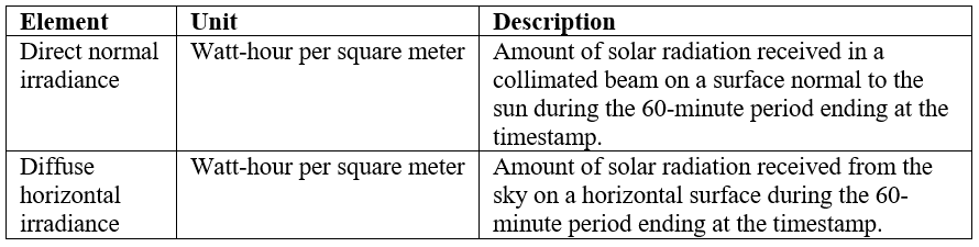
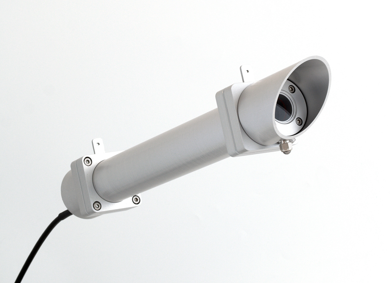
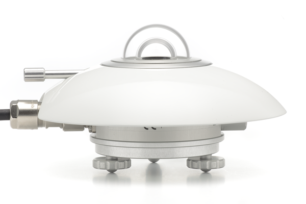
Direct normal irradiance can be measured with a pyrheliometer, an instrument that measures the solar irradiance (including visible light and ultraviolet and infrared radiation from 300 nm to 2800 nm) incident upon its thermopile sensor (Muneer 2004). The device is always aimed directly at the Sun, and it includes a narrow tube that limits its field of view to six degrees (e.g., Figure 1).

Diffuse horizontal irradiance is usually measured with a pyranometer, an instrument (such as that shown in Figure 2) that measures irradiance from the sky incident upon its horizontal thermopile sensor (Muneer 2004). A shadow band may be positioned over the sensor to obscure a six degree-wide band following the path of the Sun, although it must be moved on a regular basis throughout the year. Alternatively (and more accurately), the global horizontal irradiance can be measured without a shadow band, and the measured direct normal irradiance measurement subtracted from it to determine the diffuse horizontal irradiance (ibid).

Perhaps surprisingly, these two measurements are all that are needed to model diffuse daylight.

Perez Sky Model

Based on some 16,000 full-sky scans made from Berkeley, California, Perez et al. (1993) proposed an empirical “all weather” sky model that predicts the absolute sky luminance distribution for weather conditions ranging from clear skies to totally overcast. The only two measured input parameters are direct normal and diffuse horizontal irradiance. (The model also includes the dew point temperature as a measure of atmospheric moisture content, but this has only a minor effect on the predicted luminance distribution.)

Other all-weather sky models have been proposed, but various validations studies (e.g., Noorian et al. 2008) have shown that the Perez sky model is better than most. More important, it has been implemented in the Radiance tool gendaylit to generate a single sky luminance distribution, and in gendaymtx to generate a set of hourly sky luminance distributions for the year from a TMY3 weather data file.

It should also be noted that where TMY3 weather data include direct normal and diffuse illuminance values, they have likely been calculated from the corresponding irradiance measurements using the Perez sky model. When direct normal and diffuse horizontal illuminance values are submitted to gendaylit, it uses an undocumented iterative algorithm to estimate the original measured irradiance measurements that the Perez sky model requires.

Sky Luminance Distribution

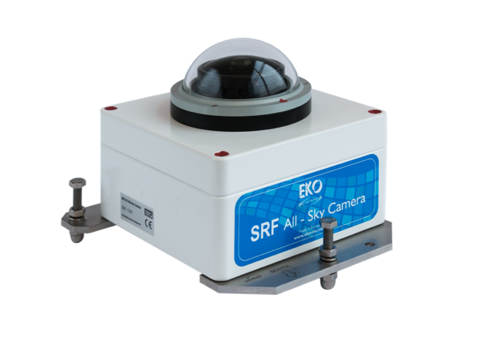
Prior to the introduction of calibrated all-sky digital cameras with fisheye lenses (e.g., Figure 3), mechanical scanners were used to measure the sky luminance distribution. Still manufactured by EKO Instruments, these instruments consist of a luminance meter mounted on an alt-azimuth platform with stepper motors, and measure the sky luminance at 145 different directions in about 4-1/2 minutes. They were previously used to obtain data for, among other purposes, the validation of various all-weather sky models, including the Perez sky model.

One legacy of these scanners has been the Tregenza sky subdivision (Tregenza 1987), wherein the sky dome is subdivided into eight 12-degree horizontal bands with 145 sky patches (Figure 4).

A particular advantage of this subdivision is that the sky luminance distribution can conveniently be represented as 145 discrete luminance values. Apart from the circumsolar region within a few degrees of the solar disk, the luminance of the sky dome in any direction can be interpolated with reasonable accuracy from these values.

Daylight Coefficients

Another advantage of the Tregenza subdivision scheme comes from a paper published over three decades ago, simply titled “Daylight Coefficients” (Tregenza et al. 1983). The researchers observed that each sky patch can be thought of as a separate and independent area light source that potentially illuminates a room through a window or opening (Figure 5). Using radiative transfer theory (aka radiosity), they demonstrated that — in theory — the luminance distribution in the room due to the intereflection of diffuse daylight from the sky patch (which they called “sky zones”) could be calculated.

Suppose, then, that each sky patch is assigned a luminance of 1000 cd/m². If the luminance distribution in the room due to each patch is calculated and the results summed, the resultant luminance distribution is that due to a uniform sky[2] with a luminance of 1000 cd/m². For the lack of any previous terminology, we can call this the canonical solution for the distribution of diffuse daylight in the environment (e.g., Figure 6).

Given, however, that each sky patch represents an independent light source, its resultant luminance distribution can be scaled by the average luminance of the sky patch for any given Perez sky model solution and building orientation. Summing these scaled luminance distributions therefore provides the luminance distribution of daylight in the room for the Perez sky model solution (e.g., Figure 7).

This is the key to climate-based daylight modeling. Given the architectural plans for a building, it is possible to calculate the canonical solution for the distribution of daylight in its rooms and other interior spaces. Then, given a TMY3 or similar weather dataset for the building site, the sky luminance distribution can be calculated for each daylight hour of the year using the Perez sky model , and with this the interior luminance distributions.

The advantage, of course, is that scaling and summing the contributions of each sky patch is much simpler and faster than calculating the canonical daylight solution. Even for complex environments with hundreds of thousands of polygonal elements, this can be done in milliseconds on a commodity desktop computer.

Again, however, this is in theory … in practice, the devil is very much in the details.

Direct Sunlight

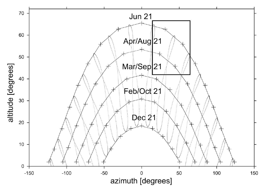
The same approach can be applied to direct sunlight. Following an approach proposed by Bourgeois et al. (2008),  interior luminance distributions can be calculated for a selected number of solar positions and included with the canonical solution (although they do not appear in the renderings). For a given TMY3 weather record, the solar position can then be calculated and the direct sunlight contribution bilinearly interpolated from the luminance distributions of the four closest precalculated solar positions.

Bourgeois et al. (2008) proposed that 65 solar positions chosen at hourly intervals on five selected days would be sufficient (Figure 8). However, choosing 120 solar positions at hourly intervals on nine selected days (Figure 9) is arguably a better choice. In particular, the average separation between solar positions is eight degrees, and the maximum separation is ten degrees. While a difference of four to five degrees may be significant in calculating the direct sunlight distribution in interior spaces for static scenes (and particularly so for photorealistic renderings), it is likely acceptable for climate-based daylight modeling where the sun traverses 15 degrees of the sky between hourly weather records. (It must also be remembered that each hourly weather record represents the average direct normal and diffuse horizontal irradiances measured over the previous hour.)

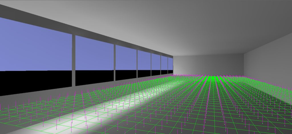
An example interior luminance distribution, including both diffuse daylight and direct sunlight, is shown in Figure 10. It should be noted that unlike ray-traced images, the shadow edges are not sharply defined. This is due to the mesh spacing of the floor (in this case 0.2 meters), and it is intentional. (This issue will be addressed in greater detail further on in this article.)

Ground Reflections

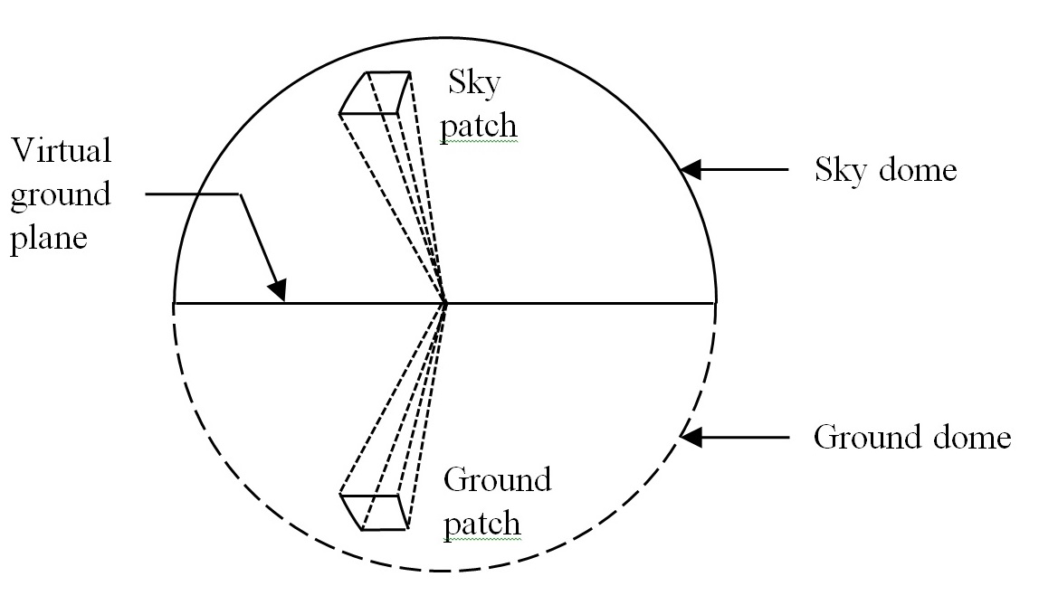
Direct sunlight and diffuse daylight reflected from the ground must also be taken into account, even if the architectural model does not include exterior surfaces. This can be accomplished by modeling a virtual ground plane as an inverted sky dome (a ground dome) with the same number of ground patches (Figure 11). Each ground patch serves the same purpose as its corresponding sky patch as an area light source. Unlike sky patches, however, all ground patches have the same luminance because they are diffusely reflecting light from the entire sky dome.

Assuming that the average reflectance of outdoor scenes is 18 percent (the same as a photographic gray card), the luminance of all ground patches is equal to 18 percent of the horizontal illuminance. Therefore, only a single interior luminance distribution needs to be determined for exterior ground reflections, which is included with the canonical solution and subsequently scaled according to the horizontal irradiance for a given TMY3 weather record.

Sky Dome Discretization

Yet another detail: most radiosity methods require all surfaces to be represented as meshes of triangular and quadrilateral elements. This is problematic in terms of the Tregenza sky subdivision, whose sky patches have curved edges. If the sky dome is represented as planar trapezoidal elements (e.g., Figure 12), the resultant gaps will result in errors of several percent or more when calculating luminance distributions due to diffuse daylight.

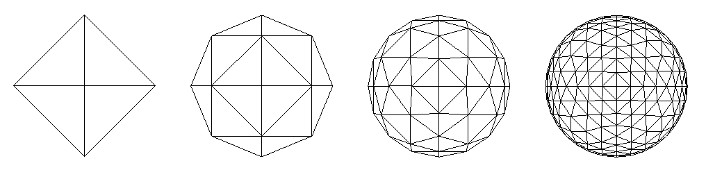
The solution is to instead represent the sky dome with a hemispherical geodesic dome. The vertex coordinates of each planar sky patch can be determined by recursively subdividing half of an octahedron, as shown in Figure 13. Three subdivisions result in a geodesic dome with 256 triangular (and, of course, planar) patches with no gaps.

With this, there is another important detail to consider. In their “Daylight Coefficients” paper, Tregenza et al. (1983) assumed that each sky patch would be projected onto a point on each surface element in the environment, as shown in Figure 5. This works in theory, but it is computationally inefficient in the extreme in that all 256 sky patches would need to be projected onto each surface element of both the interior and exterior environments. With today’s architectural models, this could involve hundreds of thousands of elements … and hours to days of computer time (e.g., Muller et al. 1995).

 Parallel Sky Patch Projection

A much more efficient approach is to model each sky patch like the solar disk, as an infinitely distant point source that produces a parallel beam of light (Ashdown 2004). With this, the sky patch illumination can be projected onto the entire environment at once, with all surface elements being considered in parallel (Figure 14). This is a standard computer graphics operation that can be performed either in software (e.g., Ashdown 1994) or in hardware using the computer’s graphics processing unit (Rushmeier et al. 1990).

This approach works well for most exterior environments because the envelopes of exterior objects (such as buildings) are typically convex. As a result, each exterior surface element is visible to multiple sky patches, with their parallel light beams being averaged and so not noticeable in the computer graphics renderings.

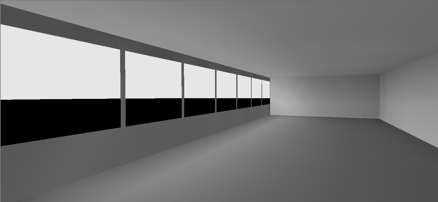
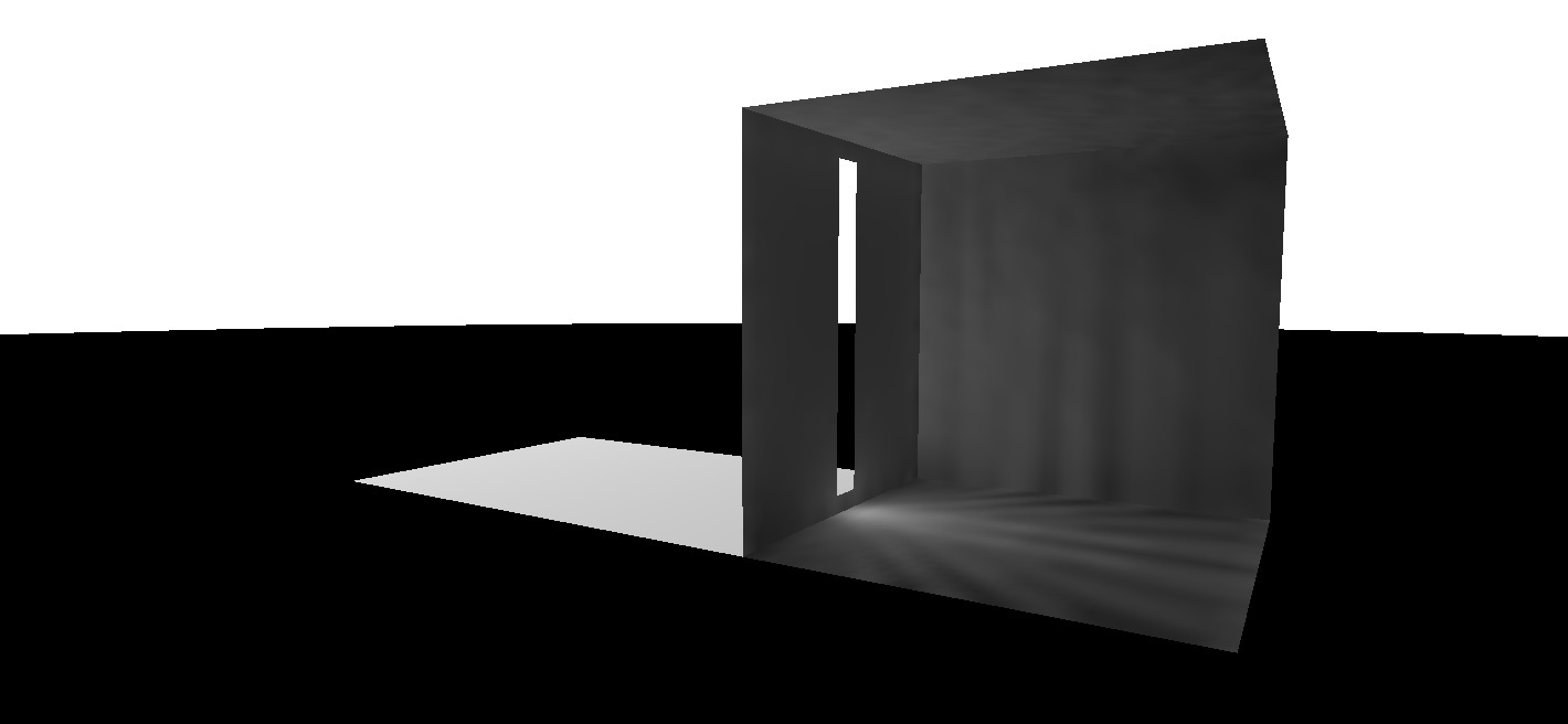
This assumption fails, however, for the windows and openings of interior environments. An example is presented in Figure 15, where the parallel light beams from the discrete sky patches are clearly visible as light “spokes” when they are projected through a narrow window onto the surfaces of interior environment.

Another problem (not illustrated here) is that the light levels in interior environments are often orders of magnitude less than the exterior horizontal illuminance. When the CAD models (such as the simple box shown in Figure 15) are specified, their surface edges may align exactly. However, when these models are rotated, translated, and possibly scaled in world space coordinates for lighting calculations, floating-point round-off of the vertex coordinates may result in very small gaps between surfaces such as the walls and floor.

(This is not a software problem — it is basically impossible to avoid this problem. Even the most high-end computer graphic displays may exhibit occasional single-pixel flickering at the surface edges when the objects are rotated or orbited for viewing.)

Even though the gaps may be fractions of a millimeter wide in world space, they allow direct sunlight or even diffuse daylight to enter the interior environment. While the amount of light is usually insignificant in terms of lighting calculations, the resultant “light leaks” can be quite obvious in computer graphics renderings.

To address these two problems, a radically different approach is needed when handling windows and openings in daylight calculations.

Windows and Openings

As previously noted, each exterior surface element is visible to multiple sky patches, with their parallel light beams being averaged. Windows are no different — they typically have a full hemispherical view of the exterior environment. Imagine then placing a camera with a fisheye lens facing outwards on the window and capturing a hemispherical image of the visible sky patches and exterior surface elements.

Comparing this to a ray tracing approach, each pixel represents a light ray that is incident upon the camera. It is slightly better than this, as the pixels each “see” a rectangular cone of light with no gaps between them. This being done in software, the camera resolution is arbitrary. With (say) 1.5 million pixels, a highly detailed high dynamic range image can be captured. The value of each pixel is the red-green-blue spectral radiance [3] in its field of view.

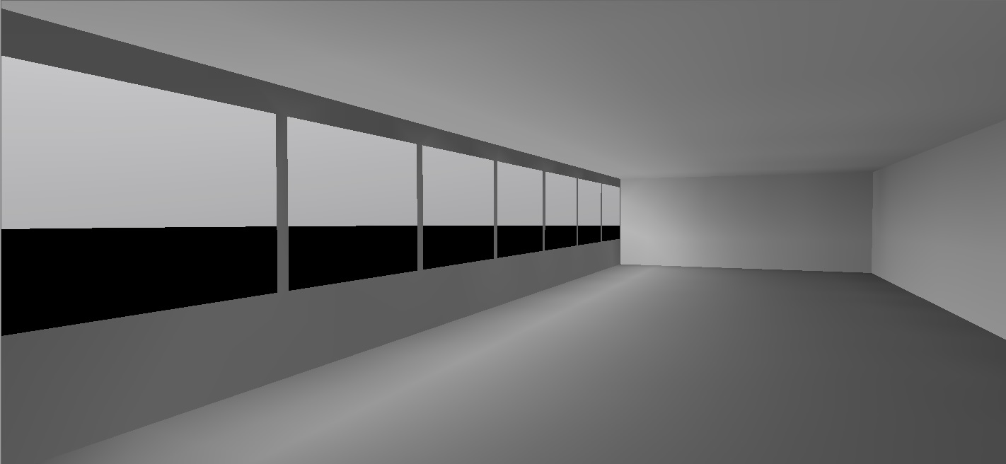
If we now reverse the camera orientation such that it faces inwards, we can project this HDR image onto the interior surface elements. This effectively transfers diffuse daylight and direct sunlight through windows and openings without the problems of light spokes, as shown in Figure 16.

The virtual camera measures the exterior spectral radiance distribution at its position on the window. At the same time, the projection of the parallel light beams from the sky patches yields the average spectral irradiance of the entire window surface. Knowing this value and the window area, the total amount of spectral radiant flux that is to be transferred through the window can be calculated.

There are, of course, further details — many of them — that need to be considered with this approach. Glass windows and transparent plastic (collectively, dielectric) surfaces exhibit complex reflectance and transmittance characteristics that vary with incidence angle (described by Fresnel equations), and may also exhibit spectrally selective absorptance (e.g., colored glass). There may also be multiple surfaces (e.g., triple-pane glazing) present. All of these issues, however, can be efficiently dealt with using radiosity-based methods.

This approach addresses the light spokes issue, but not light leaks due to floating-point round-off of the environment geometry. Solving this problem requires that the environment be separated into “exterior” and “interior” surfaces. The difference is that interior surfaces are illuminated only by daylight that is transferred through windows and openings (collectively, transition surfaces). With this approach, light leaks can be completely eliminated, no matter how imprecise the environment geometry.

Eliminating Hot Spots

There is yet another problem to consider. If we place the virtual camera at the center of a large window that is too close to an interior surface, it may result in a “hot spot” on the surface (e.g., Figure 17).

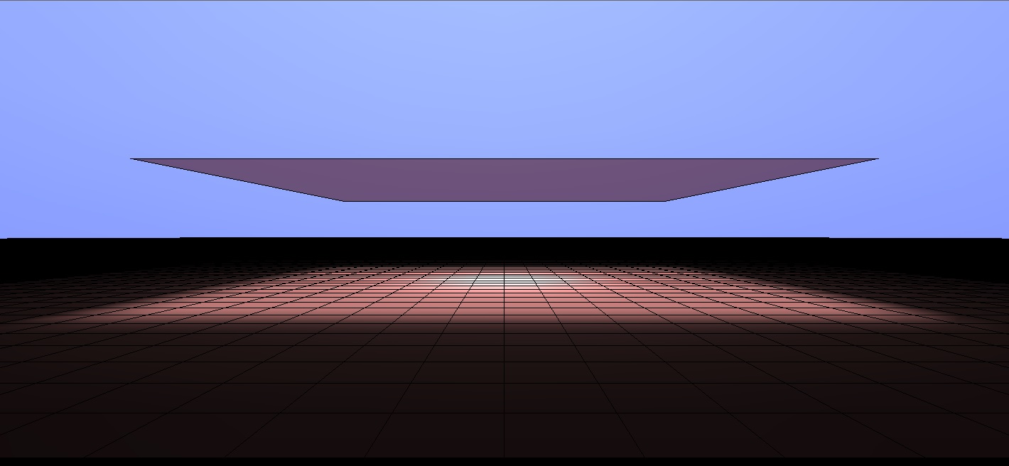
The reason for this spot is clear: the camera is concentrating all the light received by the window at a single point and projecting it onto the surface. The window is being modeled as a point source, and so the inverse square law applies.

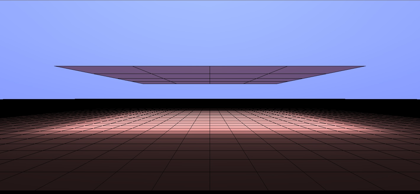
The solution is equally clear, and in fact is required by IES LM-83-12: model large windows as an array of 0.3-meter square window “patches” (IES 2012). As long as the nearest significantly large interior surface is at least 0.6 meters distant (or twice the width of each window patch), the problem of hot spots will be eliminated (e.g., Figure 18).

Annual Daylight Simulations

Without delving into the details of how the radiosity method works — see Ashdown (1994) for some 500 pages of explanation — roughly 95 percent of the calculation time involves computing form factors between surface elements for each “step” of the iterative radiosity solution (e.g., Rushmeier et al. 1990). Most of the remaining time per step is spent calculating the amount of light transferred between elements with each “bounce” of light.

With the radiosity method, each surface element is assigned a parameter that represents how much light (technically, spectral radiant exitance) it has received at each step in the calculations. Given that there are 256 sky patches, 120 solar positions, and a virtual ground plane, all that needs to be done (while blithely ignoring the myriad details) is to assign an additional 377 parameters per surface element. These are used to store the 377 separate radiosity solutions that together represent the canonical daylight solution for the environment. This requires a considerable but still manageable amount of memory for even complex environments.

The same approach can be applied to electric lighting channels, with one additional parameter per channel. This enables, for instance, the ability to model daylight harvesting systems with switched or dimmable luminaires.

The obvious question is, how quickly can these calculations be performed, particularly for complex environments with tens to hundreds of thousands of surface elements? While these are clearly empirical results, numerous experiments to date have shown that it takes between two and three times as long to calculate a canonical solution as it does to calculate an equivalent static radiosity solution for a specific date and time.

… but the devil still remains in the details …

Transition Surfaces

Looking again at the virtual cameras used to capture images of the exterior environment and project it onto the interior environment, it can be seen that each pixel needs to represent 377 spectral radiance values per pixel. Assuming a 1.5 megapixel image, this represents at least several gigabytes of memory. With a multithreaded program simultaneously processing eight to sixteen cameras, it is clear that the virtual camera approach will fail spectacularly.

The solution to this problem, however, is simple: assign a unique identifier to each surface element, which is then assigned to the pixels that “see” it in the virtual image. When the image is projected onto the interior surface elements, the identifiers can be used to access the exterior surface elements and their canonical solution values.

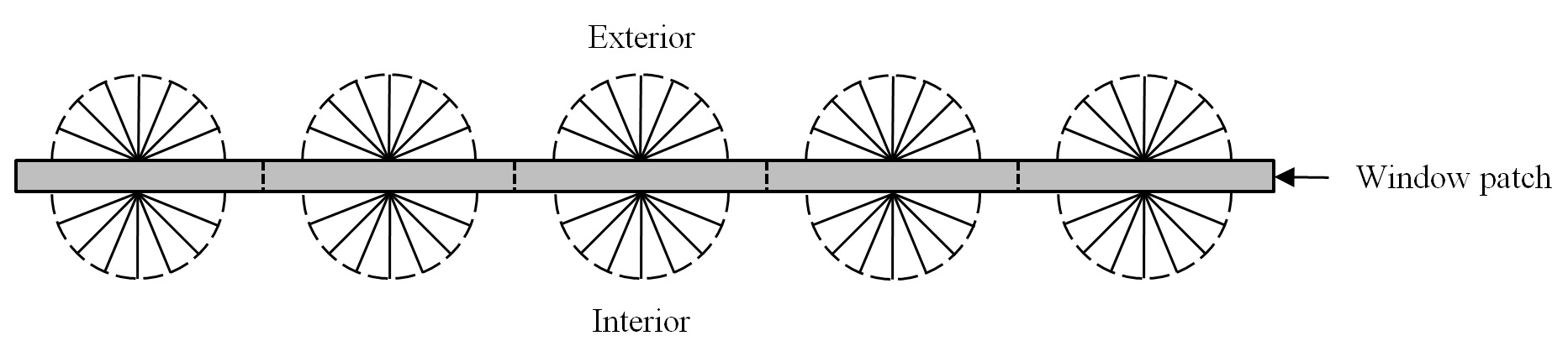
Looking more closely at windows and openings, Figure 19 diagrammatically shows virtual cameras positioned at the centers of multiple window patches, where each camera captures a hemispherical image of the exterior environment and projects the image into the interior environment.

While this approach clearly works (e.g., Figure 18), it is computationally demanding. With complex architectural models such as buildings with hundreds of windows and potentially thousands of virtual cameras, the calculation times could extend into hours.

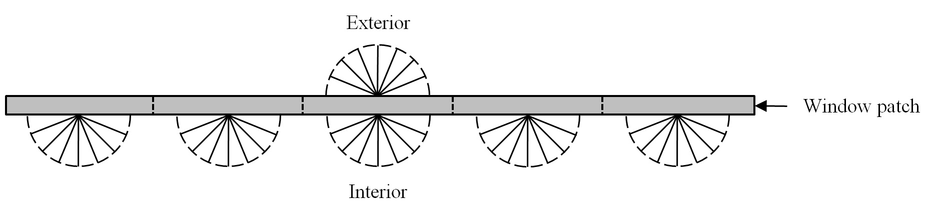
With this, it is instructive to consider again the observation that the image is equivalent to tracing a million or more rays through the camera position. With (say) a large window subdivided into one hundred 0.3-meter square window patches, this represents a dense array of 100 million light rays emanating from a single window. This may be necessary because the interior surfaces are relatively close to the window, and so the window patches are needed to avoid the formation of hot spots. For the exterior environment, however, there may not be any similarly close surfaces, and so a single virtual camera positioned in the center of the window is sufficient to capture the hemispherical image (e.g., Figure 20).

By itself, this does little to reduce the computational burden of tracing perhaps 100 million rays per window. In practice, however, as few as one million rays are likely sufficient (especially when it is considered that each ray is actually a finite width cone rather than an infinitesimally narrow ray).

The solution to this problem is to first capture the exterior image, and then randomly assign each of its pixels (i.e., rays) to one of the multiple cameras projecting the image into the interior environment. This has the effect of distributing the projected rays across the interior side of the window, which is needed to prevent the formation of hot spots. At the same time, the number of rays that need to be traced is reduced to those of a single virtual camera.

This process can be made adaptive, because each image pixel also provides the distance from the camera to the first intersected surface. By first capturing and projecting an image from the center of the window, this depth information can be used to identify the closest surfaces and so decide how best to subdivide the window on both sides (exterior and interior) for camera placement.

As complicated as this may look, it is computationally efficient. As an example, the environment shown in Figure 10 required 28 seconds of calculation time on a commodity desktop computer when calculated as a static environment for a given time and date. It is a simple environment with only 800 surface elements, but most of the calculation time is spent on transferring the direct sunlight and diffuse daylight through 84 window patches.

By comparison, the canonical solution shown in Figure 6 required only 42 seconds of calculation time. Once completed, any of the 4,380 hourly weather records in the TMY3 weather data can be calculated and displayed in milliseconds.

Bidirectional Transmittance Distribution

One of the criticisms of the radiosity approach for daylight simulation is that it can only model diffuse reflections. Quoting IES RP-5-13, Recommended Practice for Daylighting Buildings (IES 2013):

Radiosity methods assume that all surface materials have perfectly diffuse reflectance, i.e., they reflect light equally in all outgoing directions for all incident angles of incoming radiations.

This was a true statement when radiosity methods were first developed in the late 1980s, but it is certainly not true today. Radiosity methods are capable of accurately modeling the optical and spectral properties of opaque, transmissive, and translucent surfaces, including Fresnel reflectance and transmittance. They are also capable of accurately modeling both isotropic and anisotropic bidirectional reflectance and transmittance distribution functions (BRDFs and BTDFs) using analytic functions or measured data represented by the LBNL bidirectional scattering distributions function (BSDF) data format (once its specification has been finalized and published).

If commercial lighting design software has yet to support all of this functionality, it is only because there has been insufficient demand to date. IES LM-83-12 (IES 2012), however, specifies the modeling of window shades and blinds using their BSDF properties if available. Once this information become widely available from manufacturers, its simulation for CBDM purposes can be supported.

There is, however, no need to wait for measured BSDF data to become available in order to comply with the requirements of LM-83-12. Apart from advanced fenestration devices that redirect light, most diffusing glazings and fabric window shades behave as simple diffusers. Given a virtual camera, it is straightforward to include a virtual diffusion filter to model these glazings and shades.

Figure 21 illustrates several example window bidirectional transmittance distributions at incidence angles ranging from 20 to 60 degrees, and with three different degrees of diffusion. These would normally be applied to the direct sunlight entering an interior environment, but the same approach can be applied to light redirection devices such as semispecular light shelves.

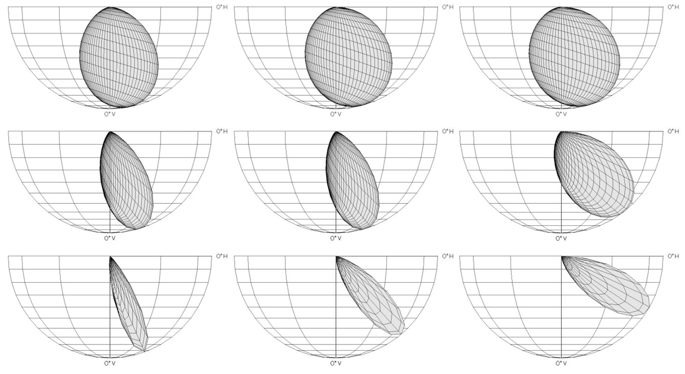
It is equally straightforward — in principle — to define a BSDF “filter” in software for the virtual camera that will redirect incident rays such that they are either transmitted or reflected by the window or other designated surface. This, however, is a work in progress for the radiosity approach.

Virtual Photometers

There is no point in calculating the distribution of daylight within an interior environment if it cannot be measured for daylight metric calculations and other purposes. Perhaps surprisingly, this is where radiosity-based CBDM has a distinct advantage over ray tracing methods.

The original radiosity methods only provided illuminance and luminance measurements for selected points on opaque surfaces after the radiosity calculations had been completed. However, it possible to extend these methods such that transparent surfaces can be specified that receive but do not otherwise influence the flow of light within the environment. By subdividing these surfaces, each surface element becomes a virtual photometer (e.g., Figure 22).

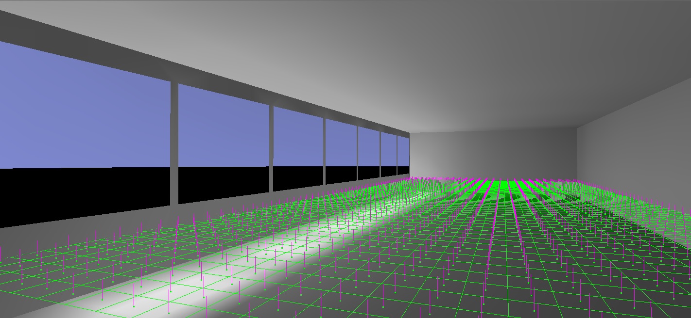
The advantage of these photometers is that they record all the light passing through them in one direction — which is exactly what is needed when performing most daylight metric calculations. By comparison, an array of photometers used in ray-traced CBDM calculations will only measure the light incident at each meter position. Depending on the resolution of the direct sunlight shadows cast by Venetian blinds, for example, those meters that are shadowed may result in the spatial Daylight Availability (sDA) and Annual Sunlight Exposure (ASE) values being underreported.

Another advantage of these photometers is that they are computationally efficient. In the above example, there are 800 surface elements and 1,500 virtual photometers placed on an imaginary workplane. Where it took 42 seconds to calculate the canonical solution without the photometers, it took 57 seconds with them. Again, this is for the canonical solution — calculating the meter values for a given TMY3 weather record is a matter of a few more milliseconds.

Looking Forward

Much of the above has been developed specifically for climate-based daylight modeling using radiosity methods. It has been implemented in commercial lighting design software, but there will undoubtedly be minor changes as users gain experience with its features and capabilities.

There are also opportunities for further improvements and optimizations, but these will not be discussed until the research and development work has been completed ñ hopefully in less time than the twelve years it has taken to reach this point!

To date, climate-based daylight modeling has relied on ray tracing methods, specifically Radiance and its derivatives. There is nothing wrong with this, other than that it has possibly hindered research into alternative approaches.

This, however, is symptomatic of a larger issue. With software products such as Lightscape in the early 1990s, radiosity methods were favored for Hollywood’s computer graphics requirements. However, the introduction of photon mapping techniques (Jensen 2001) and vastly increased computing power through “rendering farms” (thousands of dedicated computers on a network), followed by techniques such as multidimensional light cuts and Metropolis light transport, soon eclipsed radiosity methods.

Research into radiosity methods peaked in 1994 and has been declining ever since, as evidenced by the yearly total of academic papers on the topic shown in Figure 23. It is, in the terminology of computer scientists, a “solved problem.”

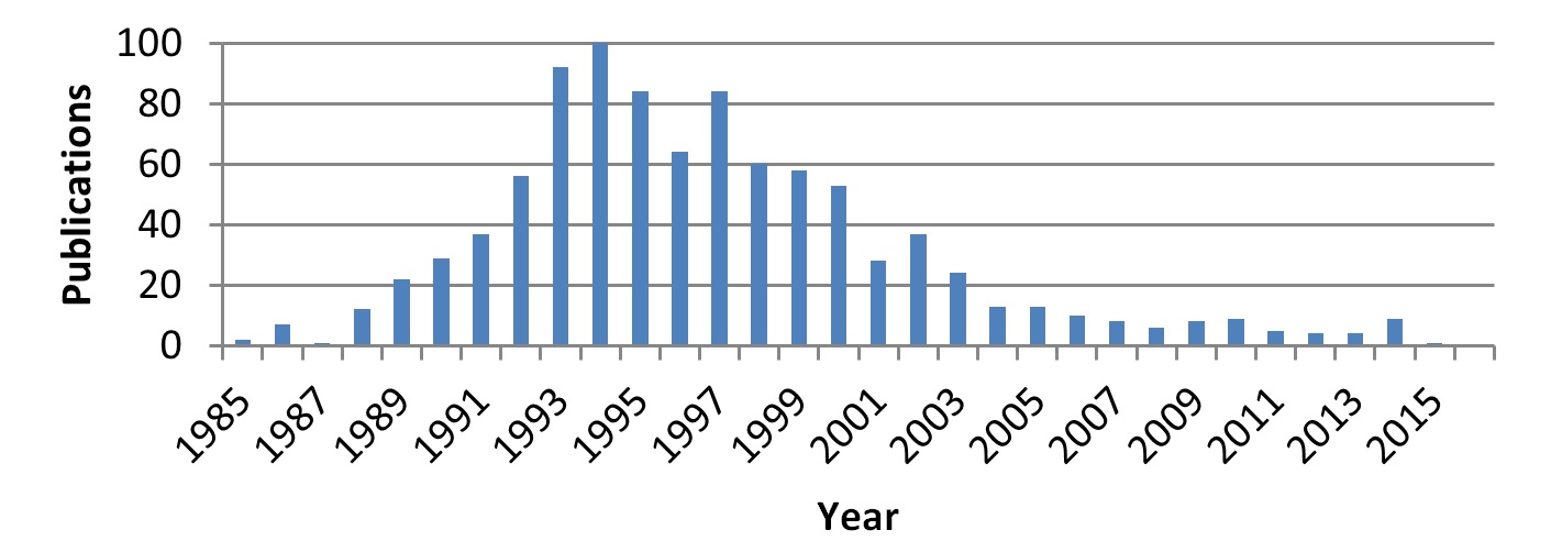
As this article has attempted to show, however, there is still life to be had in radiosity methods. As the humorist Mark Twain famously never said, “The reports of my death have been greatly exaggerated.”

Acknowledgements

Thanks to Dawn De Grazio of Lighting Analysts Inc. for her review and comments on this article.

References

1. Ashdown, I. 1994. Radiosity: A Programmer’s Perspective. New York, NY: John Wiley & Sons.
2. Ashdown, I. 2004. “Modeling Daylight for Interior Environments,” 2004 IESANZ Annual Conference Proceedings, Illuminating Engineering Society of Australia and New Zealand.
3. Bourgeois, D., C. F. Reinhart, and G. Ward. 2008. “Standard Daylight Coefficient Model for Dynamic Daylighting Simulations,” Building Research & Information 36(1):68-82.
4. CIE. 2003. Spatial Distribution of Daylight — CIE Standard General Sky, CIE Standard S 011/E:2003. Vienna, Austria: CIE Central Bureau.
5. IES. 2010. IES Lighting Handbook, Tenth Edition. New York, NY: Illuminating Engineering Society.
6. IES. 2012. LM-83-12, IES Spatial Daylight Autonomy (sDA) and Annual Sunlight Exposure (ASE). New York, NY: Illuminating Engineering Society.
7. IES. 2013. RP-5-13, Recommended Practice for Daylighting Buildings. New York, NY: Illuminating Engineering Society.
8. Jensen, H. W. 2001. Realistic Image Synthesis Using Photon Mapping. Natick, MA: A. K. Peters.
9. Mardaljevic, J. 2006. “Examples of Climate-Based Daylight Modeling,” Paper No. 67, CIBSE National Conference 2006: Engineering the Future.
10. Müller, S., W. Kresse, N. Gatenby, and F. Schaffel. 1995. “A Radiosity Approach for the Simulation of Daylight,” Rendering Techniques ’95 (Proceedings of the Sixth Eurographics Workshop on Rendering), pp. 137-146. New York, NY: Springer-Verlag.
11. Noorian, A. M, I. Moradi, and G. Kamali. 2008. “Evaluation of 12 Models to Estimate Hourly Diffuse Irradiation on Inclined Surfaces,” Renewable Energy 33:1406-1412.
12. Muneer, T. 2004. Solar Radiation and Daylight Models, Second Edition. Oxford, UK: Elsevier Butterworth-Heinemann.
13. Nabil, A., and J. Mardaljevic. 2006. “Useful Daylight Illuminances: A Replacement for Daylight Factors,” Energy and Buildings 38(7):905-913.
14. Perez, R., R. Seals, and J. Michalsky, 1993. “All-Weather Model for Sky Luminance Distribution – Preliminary Configuration and Validation,” Solar Energy 50(3):235-245.
15. Rushmeier, H. E., D. R. Baum, and D. E. Hall. 1990. “Accelerating the Hemi-Cube Algorithm for Calculating Radiation Form Factors,” ASME Journal of Heat Transfer 113:1044-1047.
16. Tregenza, P. R., and I. M. Waters. 1983. “Daylight Coefficients,” Lighting Research and Technology 15(2):65-71.
17. Tregenza, P. R. 1987. “Subdivision of the Sky Hemisphere for Luminance Measurements,” Lighting Research and Technology 19:13-14.
18. 2013. LEED v4 BD+C: Schools — Daylight. Washington, DC: U.S. Green Building Council (www.usgbc.org).
19. Wienold, J., and J. Christoffersen. 2006. “Evaluation Methods and Development of a New Glare Prediction Model for Daylight Environments with the Use of CCD Cameras,” Energy and Buildings 38:743-757.
20. Wilcox, S., and W. Marion. 2008. Users Manual for TMY3 Data Sets. Technical Report NREL/TP-581-43156, Revised May 2008.Golden, CO: National Renewable Energy Laboratory.

[1] The World Meteorological Organization (www.wmo.int) defines “climate” as the “average weather” over a period of thirty years. The weather at a given location will of course vary on a per-year basis — sometimes drastically — from that of the Typical Meteorological Year weather data for that location.

[2] A uniform sky luminance distribution is equivalent to CIE Standard General Sky Type 5 (CIE 2003).

[3] Spectral radiance in this context refers to representing visible light as a combination of red, green, and blue (RGB) light. Assuming a 6500K light source, the equivalent luminance value L is given by L = 0.2125 * R + 0.7154 * G + 0.0721 * B.