In these uncertain times, there is increasingly persuasive evidence that “far-UV” radiation is effective in inactivating the SARS-CoV-2 virus and other pathogens, but without the health risks of germicidal ultraviolet radiation. Unfortunately, this technology has some of the hallmarks of a “miracle cure,” which has become an irresistible attractant for charlatans and hucksters of all stripes.
Search the Web for “far-uv” products and you will find ultraviolet lamps, luminaires, sanitizer boxes, wands, water bottles, face masks, and more, all promising the miracle benefits of “far-uv” radiation. Look for investment opportunities online and you will find crowd-funded start-up companies clamoring to develop “far-uv” luminaires and air handling units. Search for ultraviolet germicidal irradiation (UVGI) products and you will find at least a few national companies who label every UVGI product in their catalog as “far-uv.”
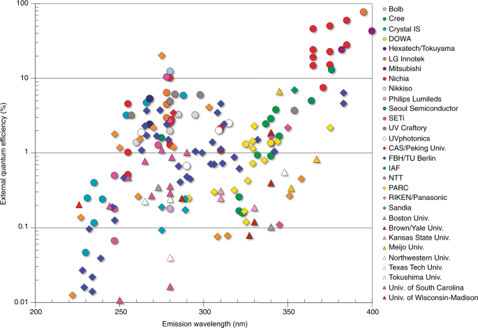
The reality is that very few of these products employ “far-uv” radiation sources. There is at present only one practical source of 222-nm UV-C radiation for germicidal applications: the krypton-chlorine excimer lamp. It is possible to manufacture light-emitting diodes with peak spectral emissions as low as 222 nm, but their radiant efficiency of slightly over 0.01 percent is abysmal (FIG. 1).
One of the problems is that “far-UV” is not what you might think it is. Read the medical literature and you will find numerous references to “far-UV,” “far-UVC,” and “far ultraviolet,” all in reference to 222 nm (and occasionally 207 nm) ultraviolet radiation sources. Scholarly publications notwithstanding however, this is incorrect. The International Lighting Vocabulary (CIE 2011) defines:
UV-A 315 – 400 nm
UV-B 280 – 315 nm
UV-C 100 – 280 nm
but with this footnote:
“In some applications the ultraviolet spectrum has also been divided into “far,” “vacuum,” and “near” ultraviolet; however, the borders necessarily vary with the application (e.g. in meteorology, optical design, photochemistry, thermal physics, etc.).”
These “some applications” include astronomy. Referring to ISO 21348:2007 (ISO 2007) regarding solar irradiances, we have:
Vacuum ultraviolet 10 – 200 nm
Extreme ultraviolet 10 – 120 nm
Far ultraviolet 120 – 200 nm
Ultraviolet C 100 – 280 nm
Middle ultraviolet 200 – 300 nm
Ultraviolet B 280 – 315 nm
Near ultraviolet 300 – 400 nm
Ultraviolet A 315 – 400 nm
The Illuminating Engineering Society follows the CIE subdivision of the ultraviolet spectrum (IES LS-1-20) under “ultraviolet subdivision,” but it also follows the ISO subdivision under “regions of the electromagnetic spectrum”:
Extreme ultraviolet 10 – 120 nm
Far ultraviolet 120 – 200 nm
Middle ultraviolet 200 – 300 nm
Near ultraviolet 300 – 400 nm
To be fair, the term “far ultraviolet” has previously defined in the academic literature to include 222-nm radiation. Forsyth et al. (1934), for example, defined:
Far ultraviolet < 270 nm
Middle ultraviolet 270 – 313.5 nm
Near ultraviolet 313.5 – 400 nm
In other words, ultraviolet-C through ultraviolet-A respectively. Suffice it to say that the definition of “far ultraviolet” has been fluid over the years.
Terminology matters. If we are to communicate effectively and unambiguously, we should respect the ISO definition of “far ultraviolet” as optical radiation with wavelengths between 120 nm and 200 nm, and refer to 222 nm radiation sources simply as ultraviolet-C emitters.
Speaking of terminology, it is ultraviolet radiation, not “light.” Light, as defined by IES LS-1-20, is “radiant energy that is capable of exciting the retina and producing a visual sensation in humans,” with wavelengths ranging from approximately 380 to 780 nm (CIE 2018). Optical radiation, on the other hand, extends from 100 nm to 1,000 mm, which includes everything from ultraviolet-C (CIE UV-C) to far infrared (CIE IR-C).
Marketing, however, will undoubtedly prevail. If 222-nm ultraviolet radiation sources become commercially important, it will be necessary to distinguish between these and the more common (and hazardous) 254-nm germicidal lamps. International standards notwithstanding, “far-UV” will be generally understood in the context of germicidal applications as optical radiation within the wavelength range of approximately 200 nm to 250 nm.
References
CIE. 2011. CIE S017/E:2011, International Lighting Vocabulary, Third Edition. Vienna, Austria; Commission Internationale de l’Eclairage.
Forsyth, W. E., et al. 1934. “Ultraviolet Source and their Radiation,” J. Optical Society of America 24(7):178-192.
IES. 2020. ANSI/IES LS-1-20, Lighting Science: Nomenclature and Definitions for Illuminating Engineering. New York, NY: Illuminating Engineering Society.
ISO. 2007. ISO 21348:2007, Space Environment (Natural and Artificial) – Process for Determining Solar Irradiances. Geneva, Switzerland: ISO Central Secretariat.
Kneissl, M. 2020. “UV-LEDs: State-of-the-Art and Applications,” in The 2020 UV Emitter Roadmap, J. Physics D: Applied Physics 53:503001.
The CIE Unified Glare Rating (UGR) metric has been use by the architectural lighting industry since it was first published by the CIE a quarter-century ago (CIE 117-1995, Discomfort Glare in Interior Lighting). Originally popularized by European lighting manufacturers, UGR has recently been adopted by the DesignLights Consortium, the US Green Building Council (LEED), and the WELL Building Standard.
It is easy enough to calculate UGR metrics using commercial lighting design and analysis programs, and luminaire manufacturers are increasingly providing UGR values for their products. However, UGR is a much more complicated metric than for example illuminance. It is the responsibility of lighting designers to *understand* the metric, rather than just blindly (no pun intended) use it in their specifications and designs.
There have been many dozens of research papers written on visual glare since CIE 117-1995 was published, but these have been of little use for day-to-day lighting design. I am therefore both pleased and proud to recommend this just-published white paper from the National Electrical Manufacturers Association (NEMA):
NEMA LS 20001-2021, White Paper on Unified Glare Rating (UGR)
UGR analysis images generated by SunTracker Technologies’Cerise365/ (c) 2021 National Electrical Manufacturers Association
I am pleased because this authoritative 34-page document “explains the original intent of Unified Glare Ratio (UGR), its proper uses, and common misuses of the Standard.” It provides detailed information on how the metric works, and how it should (and should not) be used.
I am proud because I (ahem) contributed roughly a quarter of the text, including Annex C, UGR Computer Simulations. If you *really* want to know all the gory details of how a lighting design and analysis program should calculate the UGR metric, this annex provides the answers. (Note the qualifier “should” — some programs may surprise you.)
One final comment: the white paper is free, but you have to register with NEMA in order to download it. This may be an annoyance, but I can promise that it will be worth the effort. This white paper is an essential resource for today’s lighting designers.
The phrasedéjà vutranslates from French as “already seen,” which nicely describes a current issue with horticultural lighting design. The introduction of LED technology may have kick-started horticultural lighting as an innovative industry, but we have yet to learn an important lesson from four decades of architectural lighting.
The Importance of Design Data
Prior to the 1980s, architectural lighting design was more art than science. Electrical engineers needed nothing more than pencil and paper to perform lighting calculations by hand. This all changed, of course, with the introduction of personal computers.
Today’s architectural lighting design software began with simple programs that had a particular problem. Luminaire manufacturers published plots and tables of photometric data for lighting designers, but these were useless for computer calculations.
The Illuminating Engineering Society recognized this problem, and in 1981 introduced a standardized computer file format for representing photometric data (ANSI/IES 2019). Unfortunately, the initial response of the major luminaire manufacturers was to simply ignore this development.
The argument at the time seemed reasonable enough: the published plots and tables were included in printed catalogs that sales representatives could hand-deliver to their clients. These visits generated sales opportunities that would be lost if lighting designers were able to do computer-aided calculations themselves.
Following this argument, the luminaire manufacturers mostly decided that their product data was proprietary, and that clients would be better served by requesting custom light plans through their sales representatives.
In a word (or two),déjà vu. Four decades later, this is exactly the argument that most horticultural lighting manufacturers are offering.
Failure to Communicate
The decision of architectural luminaire manufacturers to declare their product data as proprietary information was in retrospect a woeful mistake. The capabilities of lighting design software rapidly improved, giving lighting designers and engineers the ability to tackle more challenging projects, and also – critically – to compare the performance of luminaires from different manufacturers.
For lighting sales representatives in particular, it was an increasingly costly mistake. Given a choice between products for which electronic data (stored on floppy magnetic disks) was available and printed tables in catalogs, many lighting designers simply refused to specify the latter. In a competitive market driven by specification sales, this was not good.
Today, architectural luminaire manufacturers provide photometric and electrical data for virtually all of their commercial and industrial products, using industry-standard file formats such as ANSI/IES LM-63 (North America) and EULUMDAT (Europe). This downloadable information is freely and publicly available, and it is fully expected that professional lighting designers will use the data to compare the performance of products from different luminaire manufacturers.
Luminaire Design
The availability of lighting design software with visualization capabilities had a further unexpected effect on luminaire design. In being able to model the distribution of light in complex architectural environments, lighting designers could see where the light needed to go. From this, they could tell their luminaire sales representatives what they needed in terms of product performance.
Luminaire manufacturers responded by designing products with increasingly sophisticated optics, including reflectors, lenses, and holographic diffusers. The introduction of LED technology supercharged this effort because it is much easier to control the light emitted by point sources.
Horticultural Lighting
With this as historical background, it is interesting to look at the current state of horticultural lighting design. At present, not a single horticultural luminaire manufacturer offers publicly available photosynthetic photon intensity distribution (PPID) or spectral quantum distribution (SQD) information for their products. When asked, the explanation is familiar: the information is proprietary, but custom light plan services are available for qualified clients.
“It’sdéjà vuall over again,” as the baseball legend Yogi Berra probably never said.
The product information that is generally available from the manufacturers’ catalogs is rather sparse:
Photosynthetic photon flux (PPF), measured in micromoles per second per square meter;
Photosynthetic photon efficacy (PPE), measured in micromoles per Joule; and
Electrical input watts.
This is sufficient to guesstimate the number of luminaires required for a greenhouse or vertical farm, and to calculate the electrical power requirements, but nothing more.
Knowing the SQD (aka the “spectrum”) of a horticultural luminaire is an important issue, as most commercial greenhouse crops have species- and life cycle-specific responses to different SQDs (e.g., ANSI/IES 2021). If available at all, this information is presented either in graphical form in the catalog, or as “red,” “green,” and “blue” PPF values in a printed table.
It has been argued that the horticultural lighting industry does not need any more detailed information than this. While architectural lighting design programs such as Lighting Analysts’ AGi32 and DIAL’s DIALux are capable of performing basic horticultural lighting calculations, few people in the horticultural industry are interested in investing the time and effort needed to master these programs. It makes much more sense for clients to simply request custom light plans from the luminaire manufacturers.
Déjà vu… this is an echo of the arguments advanced in the 1980s, when few architectural lighting designers owned personal computers. In retrospect, telling your clients that you are smarter and more capable than they are is never a good business strategy.
Disruptive Innovation
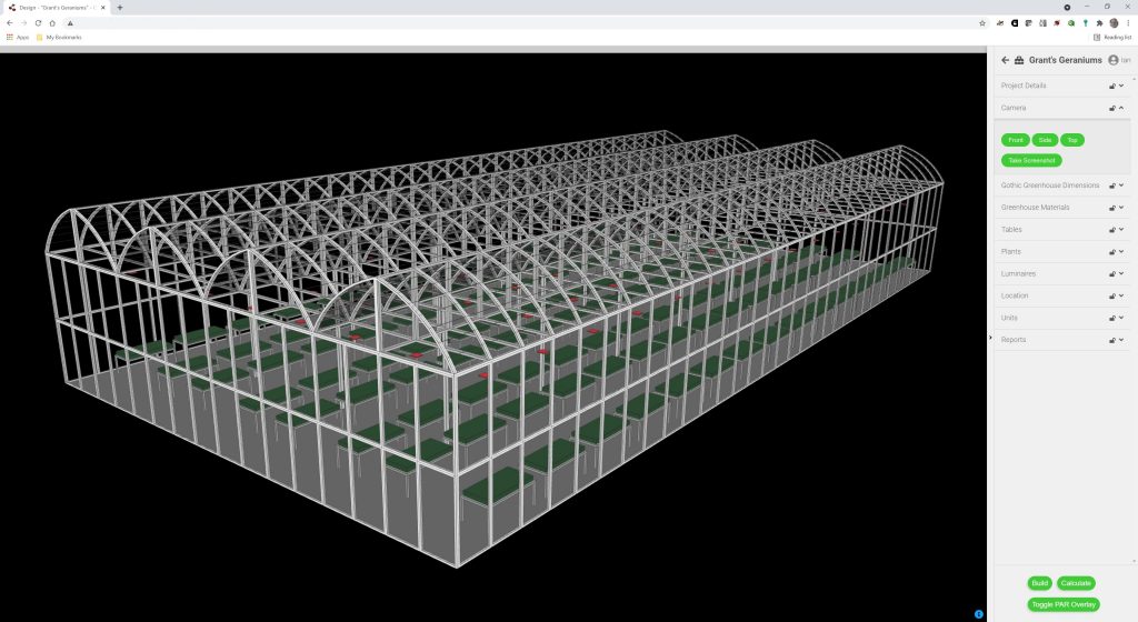
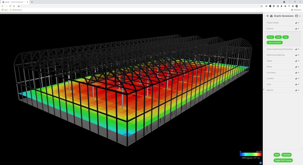
But now, consider this scenario: A professional lighting designer with computer-aided drafting (CAD) and architectural lighting design software skills is engaged to create a lighting layout for a greenhouse project. Our designer’s first task is to model the greenhouse with its luminaires, such as that shown in Figure 1.
Figure 1 – Typical greenhouse model.
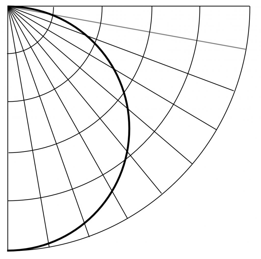
Having done this, the next task is to calculate the spatial distribution of photosynthetic photon flux density (PPFD) at the height of the plant canopy. Modeling the luminaire PPID is straightforward, as most LED-based horticultural luminaires do not employ optics and so have fully predictable cosine (“Lambertian”) PPIDs (Figure 2). If you know the luminaire PPF, the maximum PPI is PPF / π.
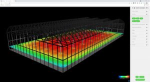
The result is shown in Figure 3, where the PPFD distribution (measured in micromoles per second per square meter) is represented by a “heat map.”
Figure 3–PPFD distribution at plant canopy.
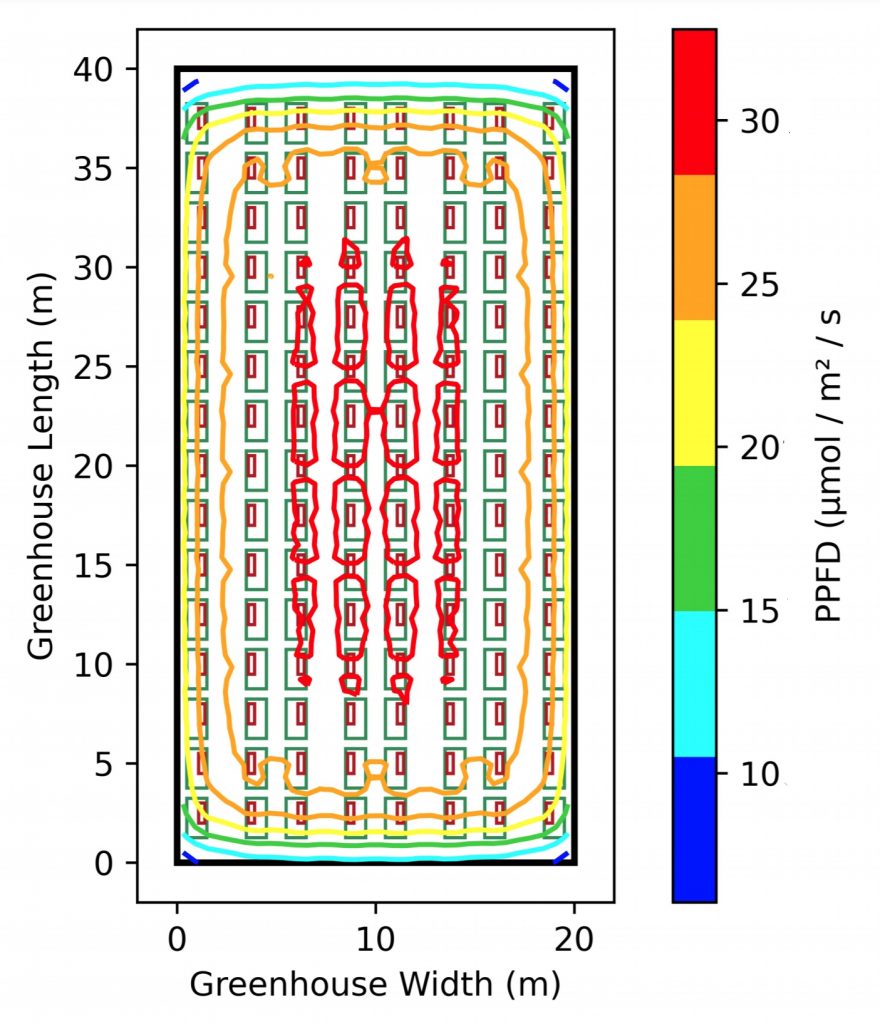
More usefully, the PPFD distribution is shown as an isoPAR plot in Figure 4.
Figure 4 – IsoPAR plot of PPFD distribution at plant canopy.
A horticulturalist may look at this heat map and realize that the distribution is uneven around the edges, resulting in poor PPFD uniformity. What the lighting designer may not know is that unlike humans, plants are particularly sensitive to differences in PPFD; a rule of thumb is that a one percent decrease in PPFD typically means a one percent decrease in the photosynthetic rate. It may also result in different flowering times for plants arranged around the greenhouse periphery. Obviously, more luminaires are needed closer to the greenhouse walls.
Our architectural lighting designer may see things quite differently. Looking at the heat map, there is clearly a need for horticultural luminaires with optical components – reflectors or lenses – to direct the light where it is needed. In this situation, it would make sense to employ luminaires with asymmetric PPIDs around the greenhouse periphery. There is no point in placing additional luminaires next to the walls if half of their light will simply escape the greenhouse entirely.
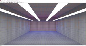
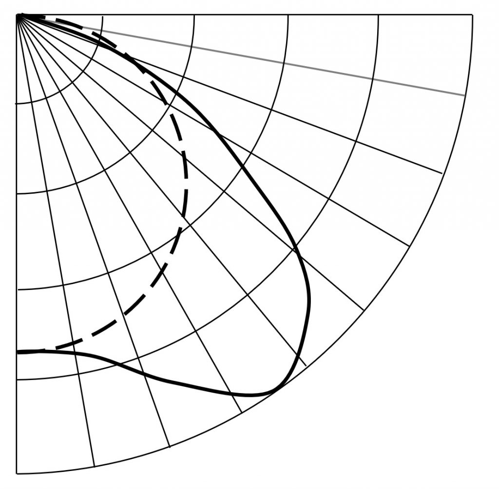
Our designer will further recognize that luminaires with “batwing” PPIDs are more efficient in achieving uniformity than today’s Lambertian distributions – the architectural lighting design community has known this for nearly a century (Figure 5). Greater uniformity means that fewer luminaires may be required.
There are at present no asymmetric-distribution luminaires for horticultural applications, and indeed few horticultural luminaires with any sort of optics. Our lighting designer may see this as an interesting business opportunity for a start-up company, possibly leading to disruptive innovation in an already crowded market with products that compete mostly on their PPE performance.
The key here is not any eureka moment on the part of our lighting designer as an industry outsider, but rather the lighting design software and accompanying luminaire optical data that made it possible to visualize the product’s performance (or lack thereof). Without such design tools, architectural lighting designers would still be working mostly with pencil and paper.
Spectral Issues
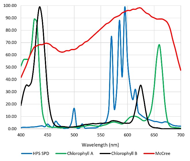
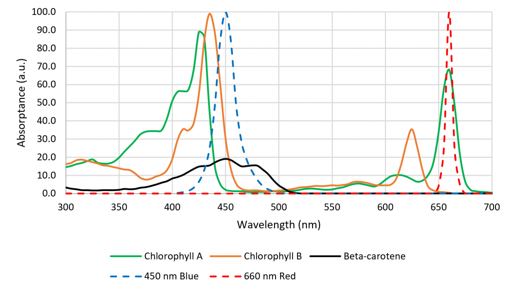
One of the tragedies of today’s horticultural lighting industry is that it is for the most part years behind academic research in terms of plant responses to the light source spectrum from 280 nm (ultraviolet-B) to 800 nm (far-red). As but one example, most luminaire manufacturers until recently offered products with only red and blue LEDs, arguing that their 450 nm (blue) and 660 nm (red) spectral outputs aligned with of the spectral absorptance peaks of chlorophyll A/B, and so would maximize photosynthesis (Figure 6).
Figure 6 – Spectral absorptance distribution of chlorophyll A/B, McCree curve, and HPS lamp spectral power distribution.
The problem with this argument is that the spectral absorptance distribution shown in Figure 6 represents chlorophyll A/B dissolved in a solvent such as ethanol (in vitro) in the laboratory. In the plant leaves (in vivo), the chlorophyll photopigments interact with accessory photopigments such as beta-carotene, resulting in a spectral absorptance distribution for photosynthesis that resembles the McCree curve. (Without this, HPS lamps would have been completely ineffective for greenhouse lighting.)
There are many more examples, including varying the red-to-far-red (R:FR) ratio on a diurnal basis for controlling plant flowering; using green light and UV-A radiation to promote secondary metabolite production; various combinations of blue, red, and yellow light to influence plant morphology … the list goes on (ANSI/IES 2021).
The point here is that luminaire spectra are of interest and potential benefit to horticulturalists. It is not enough to report the luminaire PPF as “red,” “green,” and “blue” quantities, because these colloquial terms are themselves undefined. Instead, horticultural lighting designers will need to know the detailed SQD of each luminaire, if not today then in the near future.
Some luminaire manufacturers have refused to provide any SQD data to their clients, even in graphical form, arguing that it is proprietary and confidential information. This is nonsensical, however, as anyone can measure a luminaire’s spectral output with an inexpensive spectroradiometer. However this data may be used, it will likely be inferior in quality to laboratory measurements performed by the manufacturer. At best, it will poorly represent the product’s performance in comparison with competitor’s products for which laboratory-measured data is publicly available.
DesignLights Consortium
… which brings us, somewhat indirectly, to theDesignLights Consortium(DLC®), a non-profit organization that works with utilities and government agencies to improve the energy efficiency of lighting products, horticultural lighting through their Qualified Products List.
The DLC currently has more than 450 listed horticultural lighting products from over 110 manufacturers. Most important, these product listings include PPID and SQD information, exactly what lighting designers will need when working with horticultural lighting design software.
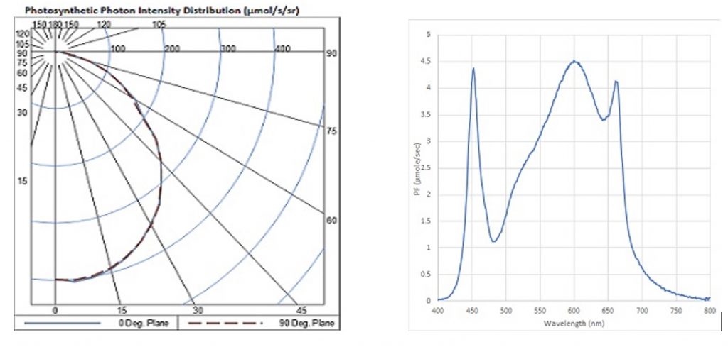
This is the good news; the bad news is that the PPID and SQD information is presented as small on-screen images, with no possibility of downloading the data for lighting design calculation purposes (Figure. 7).Déjà vu…
FIG. 7 – Typical PPID and SQD plots. (Source: www.designlights.org)
Beginning January 1st, 2022, any horticultural luminaires submitted for DLC qualification must include PPID and SQD in ANSI/IES TM-33-18 format (ANSI/IES 2018). This industry standard was specifically designed to represent optical (including PPID and SQD) and electrical data for horticultural luminaires. Moreover, it is a superset of ANSI/IES LM-63 and EULUMDAT file data.
Unfortunately, these documents will not be made publicly available by the DLC. Instead, they will be used only to generate new PPID and SQD images in a standardized presentation format. Sadly, the PPID and SQD data will remain proprietary until the horticultural luminaire manufacturers change their policies.
An Inevitable Future
Regardless of the current situation, the future of horticultural lighting design is inevitable – luminaire manufacturers will eventually have to provide PPID and SQD data for their products to lighting designers. To do otherwise is to rely on customers who purchase their products exclusively from the manufacturer without comparing their performance to that of their competitors’ products.
Some manufacturers will undoubtedly insist that they offer not only custom light plans with their proprietary data, but the knowledge and expertise of their customer support staff as well. This is a reasonable argument in an industry that is not focused exclusively on lighting design, but it is still a risk. We need only look to the past to see whether this strategy will continue to work in an open market for horticultural luminaires.
References
ANSI/IES. 2018. ANSI/IES TM-33-18, Standard for the Electronic Transfer of Luminaire Optical Data, New York, NY: Illuminating Engineering Society.
ANSI/IES. 2019. ANSI/IES LM-63-19, Approved Method: IES Standard File Format for the Electronic Transfer of Photometric Data and Related Information. New York, NY: Illuminating Engineering Society.
ANSI/IES. 2021. ANSI/IES RP-45-21, Recommended Practice: Horticultural Lighting. New York, NY: Illuminating Engineering Society.
Look at any textbook on botany and you will find this maxim: plants respond to optical radiation in the spectral range of 280 nm to 800 nm. Period, end of discussion. The question is, how was this spectral range (sometimes referred to as Photobiologically Active Radiation, or PBAR) determined?
This question addresses issues beyond mere academic curiosity. Recent studies, both in the laboratory and in the field, have shown that ultraviolet-C radiation – optical radiation with wavelengths shorter than 280 nm – offers significant economic benefits for horticultural applications. The effects and potential economic benefits of near-infrared radiation – optical radiation with wavelengths longer than 800 nm – have yet to be explored.
Ultraviolet Radiation
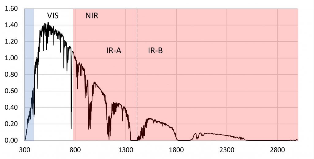
The reason for choosing 280 nm as the lower limit of PBAR is simple: plants in the wild are simply not exposed to ultraviolet-C radiation. As shown by the terrestrial solar spectrum in Figure 1, the atmospheric ozone layer effectively blocks any significant amount of ultraviolet-C radiation (100 nm to 280 nm) from reaching the Earth’s surface.
FIG. 1 – Terrestrial solar spectrum (ASTM G173-03).
The logic of excluding UV-C radiation from the definition of PBAR may be sound, but it has had unintentional consequences. We have had the ability to produce UV-C radiation for ultraviolet germicidal irradiation (UVGI) applications for over a century (e.g., Kowalski 2009), and low-pressure mercury vapor lamps generating 254 nm UV-C radiation have been used in hospitals and food processing facilities for disinfection purposes since the 1930s. However, it has only been in the past decade or so that UV-C irradiation (mostly using 254 nm UV-C lamps) has been studied and commercialized for pre- and post-harvesting applications in horticulture (e.g., Aarrout et al. 2020, Urban et al. 2016).
The use of UV-C radiation in commercial horticultural applications, including in open fields, greenhouses, and enclosed vertical farms, is proving to have important economic benefits in terms of plant health and reducing spoilage post-harvest. This therefore begs the question: by excluding near-infrared radiation (NIR) from the definition of PBAR, what (if anything) are we missing?
Far-red and the Phytochromes
To understand why 800 nm was chosen, we first need to look at the phytochromes, a class of photoreceptors that control numerous functions in higher plants, including seed germination, shade avoidance, photomorphogenesis, stem elongation, branching, circadian rhythms, root growth, and flowering times (e.g., Smith 2000 and Wang et al. 2015).
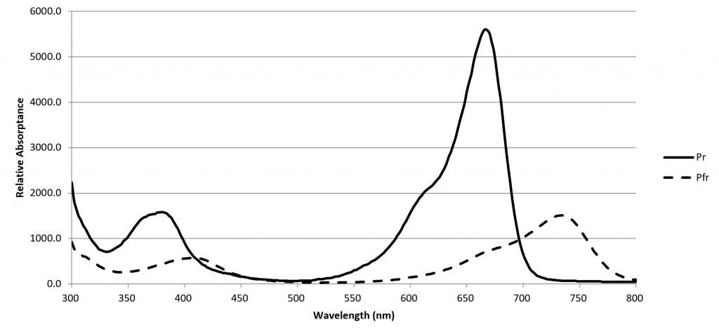
A phytochrome molecule has two isoforms, or states. Its ground state, designated Pr, preferentially absorbs red light with a peak spectral absorptance at approximately 660 nm. Upon absorbing a red photon, the molecule undergoes a conformational change to become the Pfr isoform. Left in the dark, this isoform will eventually revert to the Pr ground state. However, the molecule will also revert to the ground state if it absorbs a far-red photon with a peak spectral absorptance at approximately 725 nm.
The Pfr isoform regulates physiological changes in plants, and so it represents the biologically active form of phytochrome. It is, in other words, a biological switch. The relative concentration of Pr to Pfr will depend on the ratio of red to far-red light (expressed as R:FR) incident upon the plant leaves, and the plant will respond accordingly (although often in a species-specific manner).
The role of red and far-red light (which is nowadays defined by ASABE 2017 as the spectral region of 700 nm to 800 nm) was discovered by Borthwick et al. (1952). They determined that red light in the region of 525 nm to 700 nm promoted the germination of lettuce seeds (Lactuca sativa L.) with a peak spectral response at 660 nm, while far-red light in the region of 700 nm to 820 nm inhibited germination, with a peak spectral response of roughly 720 nm.
The spectral absorptances of Pr and Pfr were measured in vitro by Butler et al. (1964), Gardner and Graceffo (1982), and Sager et al. (1988), with moderately similar results. Today, the high-resolution (2 nm) dataset of Sager et al. is most commonly referenced.
Of note however is the spectral limit for these datasets: 800 nm. Visible light spectroradiometers typically have a spectral range of 350 nm to 800 nm. Wider spectral ranges are possible, but at the cost of reduced spectral resolution. Thus, while near-infrared spectroradiometers are available, they typically have spectral ranges on the order of 650 nm to 1100 nm. The decision therefore to define 800 nm as the limit of PBAR may have been dependent in part on the limitations of laboratory equipment.
This would not appear to be a serious issue, however, as the spectral absorptances of both Pr and Pfr clearly do not extend significantly beyond 800 nm … so why bother looking?
Near-infrared Radiation
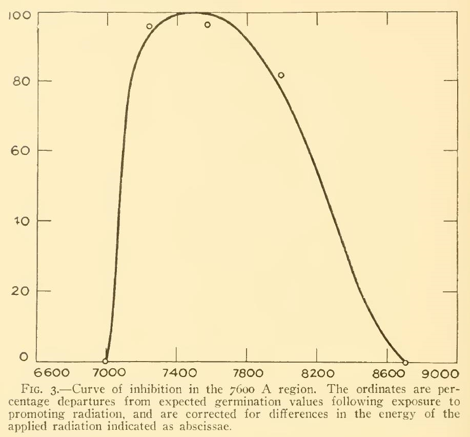
A review of the academic literature identified only three papers that considered the effect of NIR on plants. Flint and McAlister (1936) studied the effect of different spectral bands on the inhibition of lettuce seed germination, but it is unclear from their paper what data points were used to generate the plot shown in Figure 3. (The spectral bandwidth was approximately 20 nm.) Even if the small circles represent five peak wavelengths, however, the inhibition of 80 percent at 800 nm is contrary to the Pfr spectral absorptance at this wavelength.
FIG. 3 – Lettuce seed germination inhibition vs wavelength (from Flint and McAlister 1936).
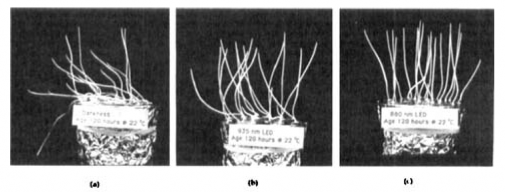
Schäfer et al. (1982) and Johnson et al. (1995) studied the effects of NIR on sprouting common oat (Avena sativa) seeds grown without visible light. Using NIR light-emitting diodes with peak wavelengths of 916 nm (nominal 880 nm) and 958 nm (nominal 935 nm), Johnson et al. noted morphological changes such as coleoptile elongation, advanced leaf emergence and increased gravitropic response (Figure 4).
FIG. 4 – Gravitropic responses of Avena sativa (common oat) seedling coleoptiles grown under: (a) darkness; (b) nominal 935 nm IR LEDs; and (c) nominal 880 nm IR LEDs (from Johnson et al. 1995).
From a horticultural perspective, these are curious but not particularly useful effects of NIR on cereal grasses grown in darkness. These studies leave the question of whether NIR has any effect on higher plants grown under electric lighting unanswered.
NIR and Daylight
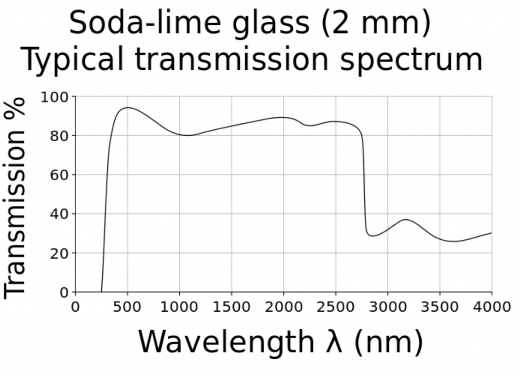
What is surprising about this question is that we should already have answers for any plant species grown in greenhouses versus the same species grown under LED lighting in vertical farms. Most greenhouse glazing is either soda-lime glass with almost constant spectral transmittance from 350 nm to 2800 nm (Figure 5), or polycarbonate panels with constant spectral transmittance from 390 nm to 1100 nm. Referring to Figure 1, the relative radiant power of the solar spectrum from 800 nm to 900 nm is 19 percent of that from 400 nm to 800 nm. The greenhouse glazing has only minimal impact on the spectral power distribution of visible light and NIR (and hence the R:FR ratio) inside the greenhouse.
In practice, however, it would be difficult to conduct experiments comparing the effects of daylight versus electric lighting. It would, for example, be necessary to match both the photosynthetic photon flux density (PPFD) and the spectral power distribution of daylight at the plant canopy. In addition, the inherent variability of daylight and consequent changes in PPFD would further complicate the experiments.
NIR and LED Grow Lights
An obvious solution is to grow plants under LED grow lights with and without additional NIR radiation sources. A 260-watt VIPARSPECTRA TC600 LED grow light system was therefore chosen to investigate the issue. This luminaire features twelve spectral bands provided by 10 quasimonochromatic and two phosphor-coated white light LEDs:
440 nm
445 nm
460 nm
475 nm
580 nm
595 nm
615 nm
620 nm
660 nm
730 nm
3000K white light
7500K white light
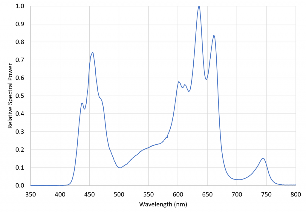
with the relative spectral power distribution, measured with a calibrated Ocean Optics STS-VIS spectroradiometer, shown in Figure 6.
FIG. 6 – VIPARSPECTRA TC600 relative spectral power distribution.
This luminaire was chosen specifically for its inclusion of 730 nm far-red LEDs. The ratio of red light (herein defined as the spectral band of 645 nm to 685 nm) to far-red light (herein defined as the spectral band of 710 nm to 750 nm), varies from approximately 1.1 in full sunlight to roughly 0.2 in the shade, where the red light is screened by the chlorophyll in the blocking leaves. The problem with most LED grow lights is that, without far-red LEDS, their R:FR ratios can be extremely high. Using a grow light with significant far-red output thus ensures that the plants are not responding to any residual PBAR emitted by the NIR radiation sources. (The VIPARSPECTRA luminaire had a R:FR ratio of 6.61.)
Petunia
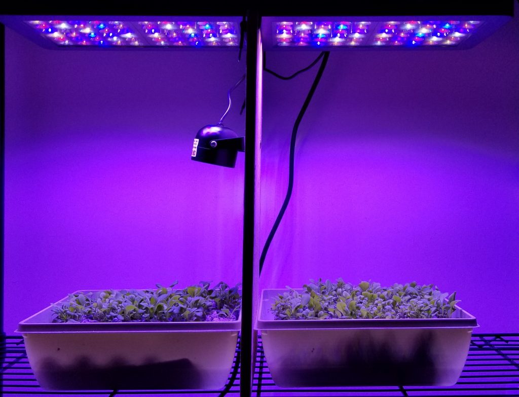
The first experiment consisted of growing petunias (Petunia x hybrida) from seed in peat moss at 20° C. The seeds sprouted in seven days under diffuse daylight before being transferred to the growth rack (Figure 7). One group of seedlings was additionally irradiated with 850 nm NIR radiation from a 4-watt Tendelux AI4 IR Illuminator with a 90-degree beam spread and an integral infrared bandpass filter. The grow light was operated with a photoperiod of 12 hours, while the NIR source was energized continuously.
A near-infrared spectroradiometer was not available to measure the spectral power distribution between 800 nm and 900 nm. However, measurements with the visible light spectroradiometer showed that any residual emission from the 850 nm LEDs below 800 nm was less than 0.3 percent of the VIPARSPECTRA peak emission.
FIG. 7 – Petunia x hybrida experimental setup.
The seedlings grown under NIR appeared to develop more quickly, but the growth rate equalized as the leaves matured after seven weeks, However, the mature leaves (8 weeks) grown under NIR were noticeably darker, suggesting a greater concentration of chlorophyll.
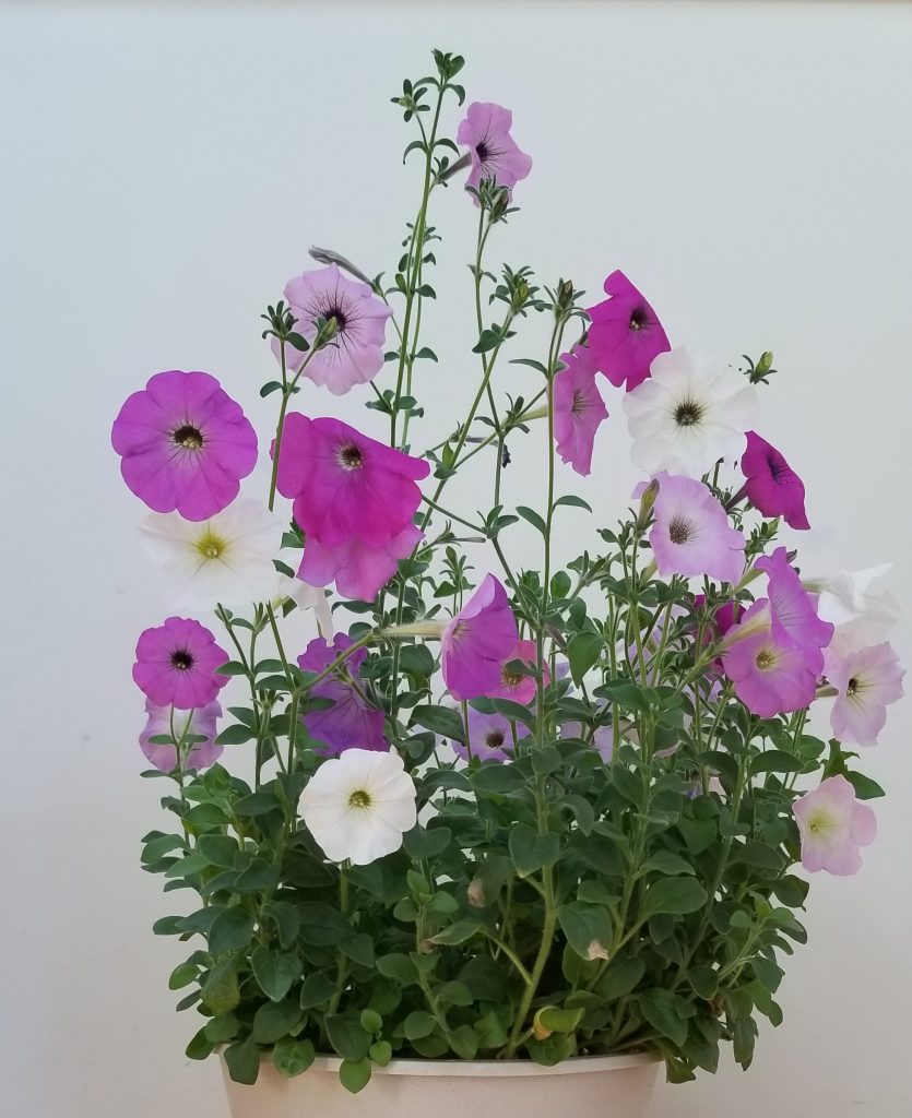
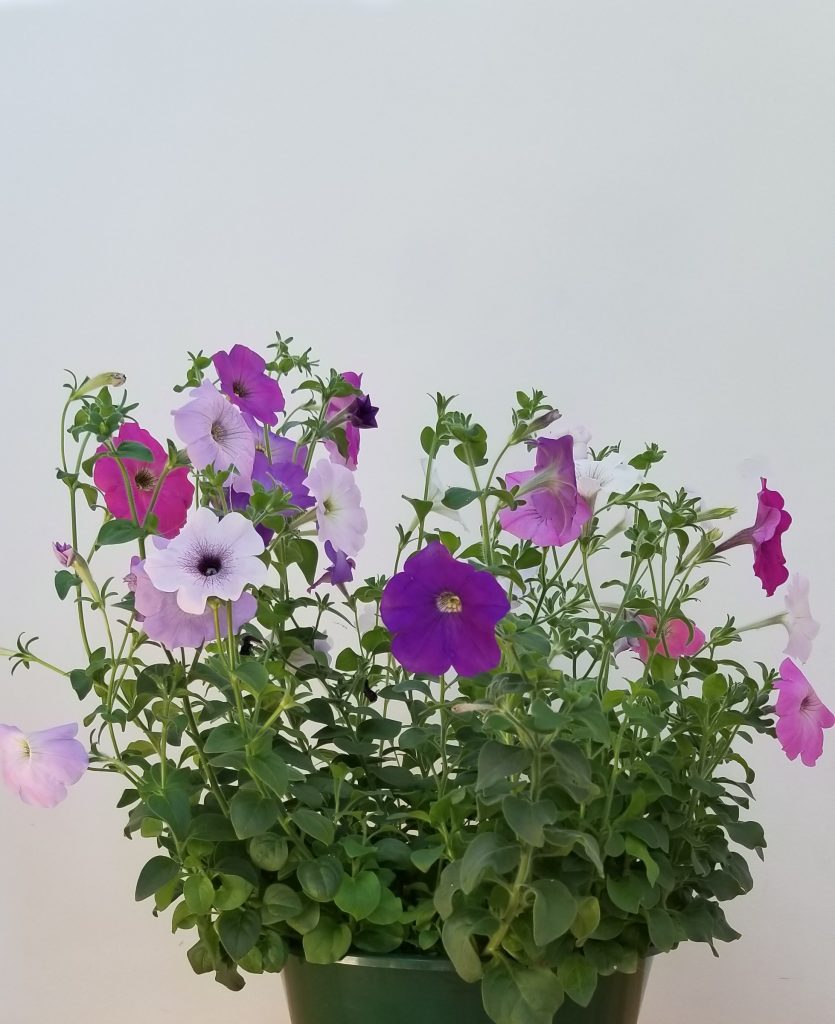
The most noticeable morphological difference was that the plants grown under NIR were considerably more compact (Figure 8).
FIG. 8A – Petunia x hybrida without NIRFig. 8B – Petunia x hybrida with 850 nm IR
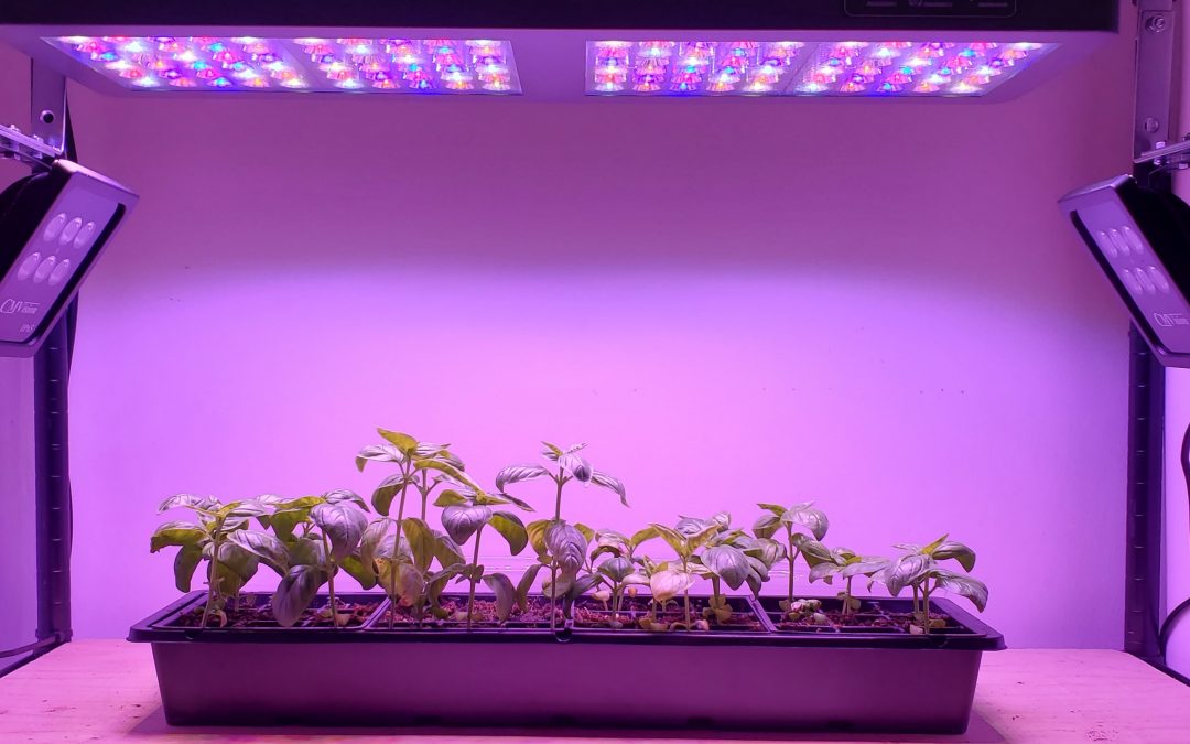
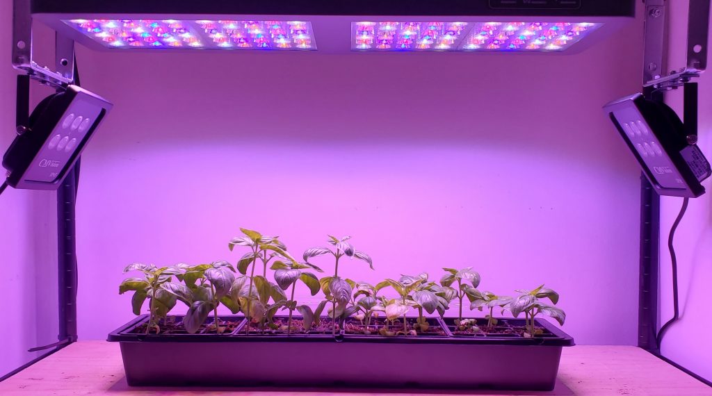
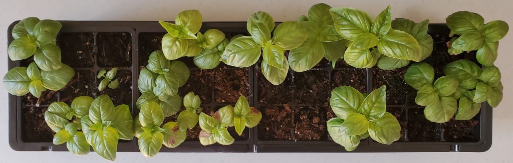
Sweet Basil
The second experiment consisted of growing sweet basil (Ocimum basilicum v. ‘Sweet Genovese’) from seed in potting soil at 20° C. Two groups were grown under separate VIPARSPECTRA grow light systems, with one group irradiated by two 18-watt CMVision CM-IRP6-850 IR illuminators with a 90-degree beam spread (Figure 9). Measurements with the visible light spectroradiometer again showed that any residual emission from the 850 nm LEDs below 800 nm was less than 0.3 percent of the VIPARSPECTRA peak emission. (The VIPARSPECTRA grow light system for the seedlings without NIR had an R:FR ratio of 7.14.)
The VIPARSPECTA grow lights were operated with a photoperiod of 12 hours, while the CMVision NIR sources were energized continuously.
Figure 9 – Ocimum basilicum experimental setup.
The seeds without NIR irradiation germinated within one week, with a success rate of approximately 50 percent. However, the seeds with NIR irradiation germinated within two weeks, and with a success rate of approximately 35 percent.
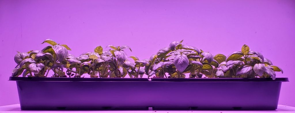
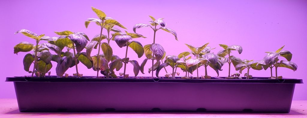
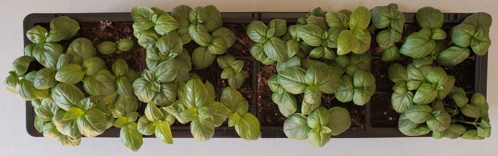
After six weeks, there was a marked difference in stem elongation, where the plants with NIR irradiation were approximately twice as tall (Figures 10A and 10B). In addition, the plants with NIR irradiation had larger and lighter-colored leaves (Figures 11A and 11B).
FIG. 10A –Ocimum basilicum without NIR (six weeks), side view.Figure 10B – Ocimum basilicum with 850 nm IR (six weeks), side view.FIG. 11A – Ocimum basilicum without NIR (six weeks), top view.Figure 11B – Ocimum basilicum with 850 nm IR (six weeks), top view.
Conclusions
Due to the lack of quantitative spectral power distributions for the NIR irradiation of the plant canopy and the differences in NIR irradiance between the two experiments, the results observed above must be considered incomplete pending further study. However, a number of tentative conclusions can be drawn regarding constant 850 nm irradiation:
Germination of Ocimum basilicum seeds is inhibited.
The shade avoidance response of Petunia x hybrida appears to antagonized, resulting in a more compact plant architecture.
The shade avoidance response of Ocimum basilicum is clearly promoted, resulting in stem elongation and thus taller plants.
The leaf area of Ocimum basilicum is increased.
The chlorophyll production in the leaves of Petunia x hybrida appears to be slightly increased.
The chlorophyll production in the leaves of Ocimum basilicum appears to be moderately inhibited.
One possible explanation for these observations is that the biologically active isoform of phytochrome (Pfr) has an unreported spectral absorption band in the region of 800 nm to 900 nm. This would have the effect of reducing the Pfr content in the leaves, which in turn reduces the chlorophyll concentration (e.g., Kreslavski et al. 2018) and increases the leaf area (e.g., Boccalandro et al. 2009). This could explain the Ocimum basilicum results, but not the Petunia x hybrida results.
NIR absorption by phytochrome Pfr could further explain the inhibition of Ocimum basilicum seed germination, as demonstrated by Flint et al. (1936) and Borthwick et al. (1952) with far-red light.
The shade avoidance response of Ocimum basilicum can also be explained by NIR absorption, as this is equivalent to lowering the R:FR ratio. The plant stems will then elongate in order for the upper leaves to receive as much full sunlight as possible.
This does not, however, explain the apparent antagonism of the shade avoidance response of Petunia x hybrida. One possibility is that the lower NIR irradiance used in the experiment elicits a nonlinear response by phytochrome Pfr, although this would be more likely to have a null rather than a negative effect.
Another possibility is that there is an undiscovered photopigment with a spectral absorption band beyond 800 nm (Johnson et al. 1995). Alternatively, there may be an undiscovered spectral absorption band in one of the cryptochromes or other known photopigments involved in photomorphogenesis.
Whatever the case, it is evident that more research is required. The PBAR limit of 800 nm has been assumed for at least the past seven decades, but then the effects of UV-C radiation on plants remained unexplored for an equal length of time. The effect of near-infrared radiation of plants is a topic that deserves to be explored.
References
ASABE. 2017. ANSI/ASABE S640 JUL2017, Quantities and Units of Electromagnetic Radiation for Plants (Photosynthetic Organisms). St. Joseph, MI: American Society of Agricultural and Biological Engineers.
Aarrout, J., and L. Urban. 2020. “Flashes of UV-C Light: An Innovative Method for Stimulating Plant Defenses,” PLoS ONE 15(7):e0235918. DOI: 10.1371/journal.pone.0235918.
ASTM International. ASTM G173-03(2020), Standard Tables for Reference Solar Spectral Irradiances: Direct Normal and Hemispherical on 37° Tilted Surface. West Conshohocken, PA: ASTM International; 2020.
Boccalandro, H. E., et al. 2009. “Phytochrome B Enhances Photosynthesis at the Expense of Water-Use Efficiency in Arabidopsis,” Plant Physiology 150(2):1093-1092. DOI: 10.1104/pp.109.135509.
Borthwick, et al. 1952. “A Reversible Photoreaction Controlling Seed Germination,” Proceedings of the National Academy of Science 38:662–666. DOI: 10.1073/pnas.38.8.662.
Butler, W. L., et al. 1964. “Action Spectra of Phytochrome in vitro,” Photochemistry and Photobiology 3(4):521-528. DOI: 10.1111/j.1751-1097.1964.tb08171.x.
Flint, L. H., and E. D. McAlister. 1936. “Wave Lengths of Radiation in the Visible Spectrum Inhibiting the Germination of Light-Sensitive Lettuce Seed,” Smithsonian Miscellaneous Collections 94(5):1-11.
Gardner, G., and M. Graceffo. 1982. “The Use of a Computerized Spectroradiometer to Predict Phytochrome Photoequilibria under Polychromatic Irradiation,” Photochemistry and Photobiology 36(3):349-354. DOI: 10.1111/j.1751-1097.1982.tb04385.x.
Kowalski, W. 2009. Ultraviolet Germicidal Irradiation Handbook: UVGI for Air and Surface Disinfection. Berlin, Germany: Springer-Verlag.
Kreslavski, V. D., et al. 2018. “The Impact of the Phytochromes on Photosynthetic Processes,” BBA – Bioenergetics 1859:400-408. DOI: 10.1016/j.bbabio.2018.03.003.
Kusuma, P., and B. Bugbee. 2021. “Far-red Fraction: An Improved Metric for Characterizing Phytochrome Effects on Morphology,” J. American Society of Horticultural Scientists 146(1):3-13. DOI: 10.21273/JASHS05002-20.
Sager, J. C., et al. 1988. “Photosynthetic Efficiency and Phytochrome Photoequilibria Determination Using Spectral Data,” Trans. ASAE 31(6):1882-1889.
Schäfer, E., et al. 1972. “In vivo Measurement of the Phytochrome Photostationary State in Far Red Light,” Photochemistry and Photobiology 15(5):457-464. DOI: 10.1111/j.1751-1097.1972.tb06257.x.
Smith, H. 2000. “Phytochromes and Light Signal Perception by Plants – An Emerging Synthesis,” Nature 407:585-591. DOI: 10.1038/35036500.
Urban, L., et al. 2016. “Understanding the Physiological Effects of UV-C Light and Exploiting its Agronomic Potential Before and After Harvest,” Plant Physiology and Biochemistry 105:1-11. DOI: 10.1016/j.plaphy.2016.04.004.
Wang, H., et al. 2015. “Phytochrome Signaling: Time to Tighten Up the Loose Ends,” Molecular Plant 8:540-551. DOI: 10.1016/j.molp.2014.11.021.
Whereas human vision relies on five opsins as photoreceptors, most plants have a wide variety of photopigments that are responsive to optical radiation from 280 nm to 800 nm. Beyond photosynthesis, plants rely on this radiation to control photomorphogenesis, phototropism, shade avoidance, and both circadian and circannual rhythm entrainment.
Quasimonochromatic LEDs have proven a boon for botanists in that the molecular genetics of these responses can be elucidated with precisely controlled spectral power distributions (SPDs). In terms of photopigments, cryptochromes, for example, respond to blue light, while phytochrome responds to the R:FR ratio of red (approximately 660 nm) to far-red (approx. 735 nm) light.
The problem is that botanists do not define what is meant by “blue,” “green,” “yellow,” “red,” or “far-red” visible light, while ultraviolet radiation is broadly defined as UV-A and UV-B. Consequently, it is difficult to replicate laboratory experiments without knowing the SPD of the horticultural light source.
This paper proposes an LED “color” specification that represents a given SPD using a small number of radial basis functions, to provide a metric for comparing biologically similar SPDs. It further introduces a trainable fuzzy logic SPD classifier that can compare biologically similar SPDs for specific horticultural applications.
Introduction
When the first high-pressure sodium (HPS) lamps were introduced in the late 1960s, they were quickly adopted by commercial greenhouse operators as a means of providing supplemental electric lighting. This made it economically possible to grow vegetables and flowers throughout the year in controlled environments. They had luminous efficacies, ranging from 100 to 150 lumens per watt, they were available in sizes ranging from 400 to 1,000 watts, and they could be incorporated in luminaire housings designed to withstand the heat and humidity of greenhouses.
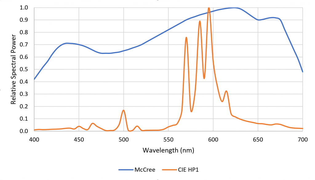
One disadvantage of HPS lamps is they produce mostly yellow light with fixed spectral power distributions (SPDs). This is not particularly important for plant photosynthesis, as most plants can take advantage of optical radiation within the spectral range of 400 to 700 nm. Horticulturalists often refer to the “McCree curve,” which plots average photosynthesis efficiency versus wavelength for a variety of field-grown crops (McCree 1972). As shown in Figure 1, the spectral output of HPS lamps is near the peak of the McCree curve.
Figure 1. Typical HPS lamp spectral power distribution versus McCree curve.
The problem is that while the yellow light of HPS lamps may be good for photosynthesis, plants have a wide range of photopigments that respond to optical radiation from 280 nm to 800 nm (often referred to as “photobiologically active radiation,” or PBAR). These responses include:
Photomorphogenesis – any change in the morphology (i.e., shape) or composition of a plant or its components that is induced by optical-radiation exposure
Photoperiodism – response of a plant to daily (circadian) or seasonal (circannual) changes in optical-radiation exposure
Photosynthesis – conversion of “photosynthetically active radiation” (PAR) into chemical energy stored as carbohydrates to fuel plant activities
Phototropism – any self-actuated change in the orientation of a plant or its components toward or away from optical radiation
Secondary metabolite production – organic compounds not directly involved in plant growth, development, or reproduction, including compounds used as medicines, flavorings, pigments, and drugs
Shade avoidance – a set of responses to being shaded by other plants, including changes in morphology, flowering times, and allocation of resources
While many of these responses have been known or suspected for decades, it was difficult for botanists to study them in the laboratory without suitable light sources. This changed, however, with the introduction of horticultural luminaires with high-flux quasimonochromatic light-emitting diodes (LEDs). Somewhat serendipitously, the absorption spectra of chlorophyll A and B have peaks that correspond with those of approximately 450-nm InGaN and approx. 660-nm AlInGaP LEDs (Figure 2). Today, the photon efficacy (measured in micromoles of PAR photons per Joule, rather than in lumens) of LED modules is typically greater than equivalent 1,000-watt HPS lamps.
Figure 2. Chlorophyll and b-carotene absorption spectra.
While commercially available horticultural luminaires with blue and red LEDs (producing so-called “blurple” light) are now successfully competing with traditional HPS luminaires, botanists’ attention has turned to the capabilities of multichannel LED luminaires with controllable SPDs. Over 500 academic studies over the past decade have investigated the effects of different wavelength ranges on plants and their absorption by photopigments (Table 1).
Wavelength Range
Color Name
Photopigments
Responses
280 nm – 315 nm
UV-B
UVR-8
Sec. metabolism Shade avoidance Phototropism
315 nm – 400 nm
UV-A
Chlorophylls Cryptochromes Phototropin Phytochromes Zeitlupe family
Sec. metabolism Photomorphogenesis
400 nm – 500 nm
Blue
Carotenes Chlorophylls Cryptochromes Phytochromes Zeitlupe family
Photosynthesis Sec. metabolism Shade avoidance Phototropism Photoperiodism
500 nm – 575 nm
Green
Cryptochromes
Photosynthesis Sec. metabolism Shade avoidance
575 nm – 610 nm
Yellow – orange
<Unknown>
Photosynthesis Sec. metabolism
610 nm – 700 nm
Red
Chlorophylls Phytochromes
Photosynthesis Photomorphogenesis Sec. metabolism Shade avoidance Photoperiodism
700 nm – 800 nm
Far-red
Phytochromes
Photomorphogenesis Shade avoidance Photoperiodism
Table 1 – Plant Responses to Optical Radiation
The problem is that while UV-A and UV-B are formally defined in the scientific literature (e.g., ISO 2007), the visible color names are colloquial and based on human visual responses. The title of one paper in particular illustrates this issue: “Green light drives leaf photosynthesis more efficiently than red light in strong white light: Revisiting the enigmatic question of why leaves are green” (Terashima 2009). For anyone interested in either replicating the experiments or extrapolating their results, what are “green,” “red,” and “white” light?
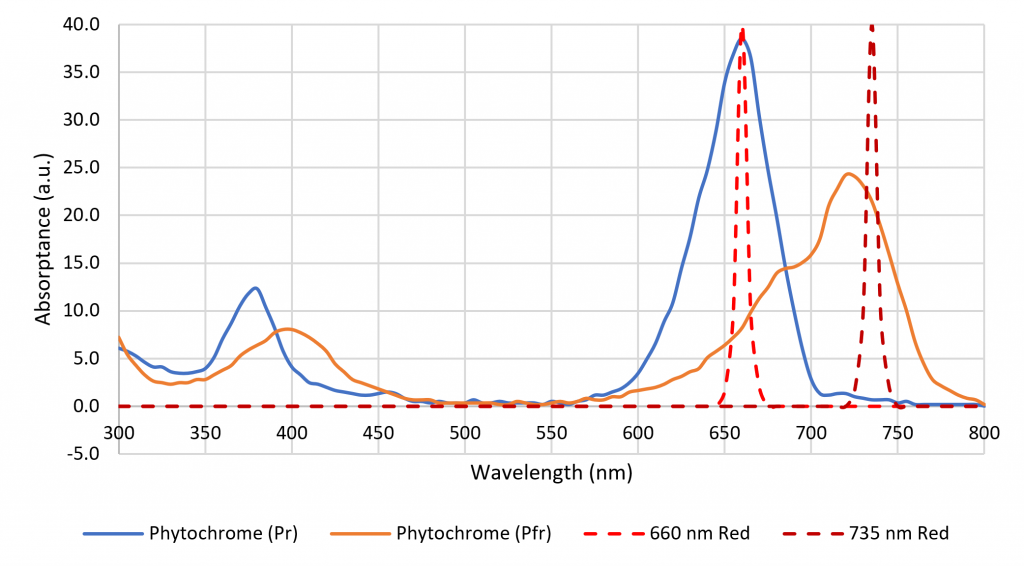
The color name “far red,” which refers to the spectral range of 700 nm to 800 nm, is formally defined in terms of horticulture (ASABE 2017). It is important in terms of shade avoidance and photoperiodism, where plants rely on two isoforms of phytochrome to detect the ratio of red to far red (R:FR) optical radiation (Sager et al. 1988), but there is no equivalent definition of “red” (Figure 3). Luminaire manufacturers are now offering products with 660-nm red and 735-nm far-red LEDs to induce or delay flowering in ornamental plants (e.g., Craig and Runkle 2013), but many previous horticultural studies have relied on daylight alone or daylight and incandescent lamps to explore the effects of varying R:FR. How should these studies be interpreted in terms of modern horticultural lighting practices with LED-based luminaires?
Figure 3. Phytochrome absorption spectra.
Characterizing SPDs
Horticultural researchers have recognized that the use of colloquial color names is a problem. Many papers describe their experimental methods in detail, including light source SPD plots, names of specific luminaire products, and occasionally tabulated SPDs. This still leaves open, however, the problem of interpreting the results in terms of other optical radiation sources with similar SPDs.
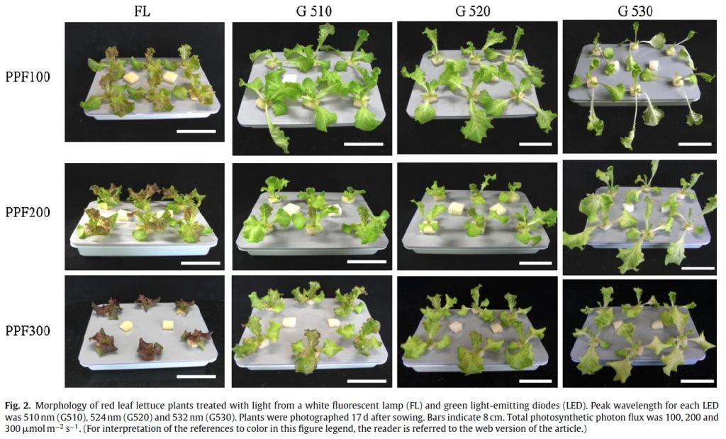
One proposed product label for horticultural light sources is shown in Figure 4 (Both et al. 2017). By avoiding the use of color names, this proposal eliminates any dependence on the human visual system. However, the arbitrary separation of the PBAR spectral range into 100-nm wide bands ignores the distinct responses of plants to UV-A and UV-B radiation, as well as the response of plants to narrower changes in wavelength. For example, Johkan et al. (2012) provide an example wherein the growth of lettuce under quasimonochromatic radiation from “green” LEDs with center wavelengths of 510 nm, 520 nm, and 530 nm varies markedly depending on the center wavelength for the same photosynthetic photon flux density (Figure 5).
Figure 4. Proposed product label. (Source: Both et al. 2017)Figure 5. Morphology of red leaf lettuce plants treated with light from a white fluorescent lamp (FL) and green light-emitting diodes (LED). Peak wavelength for each LED was 510 nm (G510), 524 nm (G520), and 532 (G530). Plants were photographed 17 d after sowing. Bars indicate 8 cm. Total photosynthetic photon flux was 100, 200, and 300 μmol·m-2·s-1. (Source: Johkan et al. 2013, Fig. 2).
The spectral absorptance characteristics of the primary plant photopigments chlorophyll A and B, b-carotene, and phytochrome (Figure 2) suggest that their absorptances vary very rapidly with changes in wavelength. However, these data represent the spectral absorptance of the pigment extracts dissolved in solvents (i.e., in vitro). As shown by Moss and Lewis (1952), a combination of the structural complexity of the leaves, screening by other photopigments, and the presence of accessory photopigments have the effect of broadening the spectral absorptance characteristics of the photopigments in vivo. Studies such as those of McCree (1972) have shown that in general, plants are reasonably tolerant of small changes in the center wavelengths of quasimonochromatic radiation. (Johkan et al. [2012] was likely an exception in that photosynthesis probably occurred due to b-carotene rather than chlorophyll A or B, with longer wavelengths of green light being incapable of exciting this photopigment.)
In view of this and other studies, it is clear that any attempt to characterize the SPDs of horticultural luminaires needs to take into consideration the responses of plants to changes in center wavelength of quasimonochromatic light sources, and more generally to horticultural luminaires with both quasimonochromatic and broadband radiation sources.
In relation to this, Maloney (1986) discusses the physical basis of spectral reflectance distributions from natural objects, including organic materials. These distributions are band-limited by molecular interactions and superimposed vibrational and rotational patterns, with the result that the number of parameters needed to adequately represent spectral reflectance distributions in visible light (i.e., 400 nm to 700 nm) is five to seven. Westland et al. (2000) came to a similar conclusion based on statistical studies of reflectance spectra, noting that the spectral reflectance distributions of most natural surfaces form a set of band-limited functions with a frequency limit of approximately 0.02 cycles per nm. This implies that visible light reflectance spectra can be adequately represented using six to 12 basis functions (e.g., Westland and Ripamonti 2004).
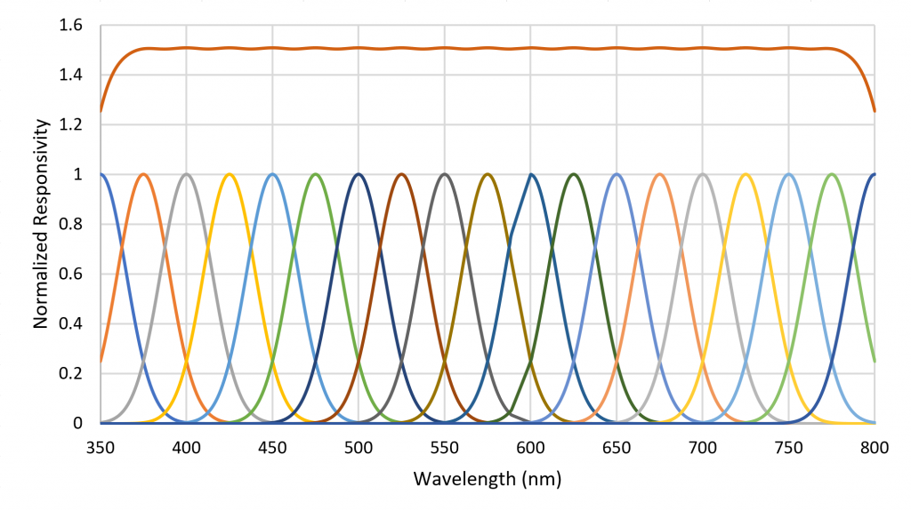
A small number of radial basis functions (e.g., Buhmann and Jäger 2000) can therefore be used to approximate a real-valued function (such as an SPD) as a weighted sum of the basis functions. As an example, the set of Gaussian functions , where , and for , can be used to approximate any SPD from 350 nm to 800 nm where the functions are separated by 25 nm (Figure 6).
Figure 6. Sum of Gaussian radial basis functions provide flat spectral sensor response.
An advantage of this method is that the set of basis function weights is much smaller than the set of enumerated values for a measured SPD. Rather than referring to “red,” “green,” “blue,” or “white” light, horticulturalists can state the values of a set of basis function weights. Moreover, a useful approximation of the original SPD significant to the needs of horticultural lighting can be reconstructed from these weights.
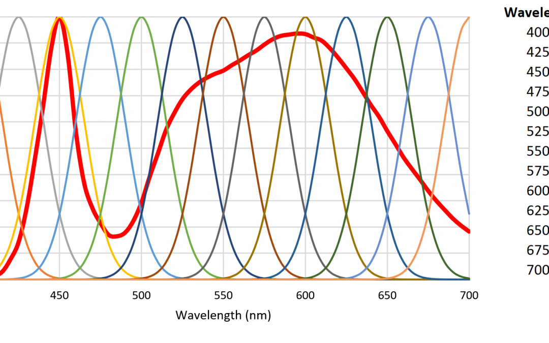
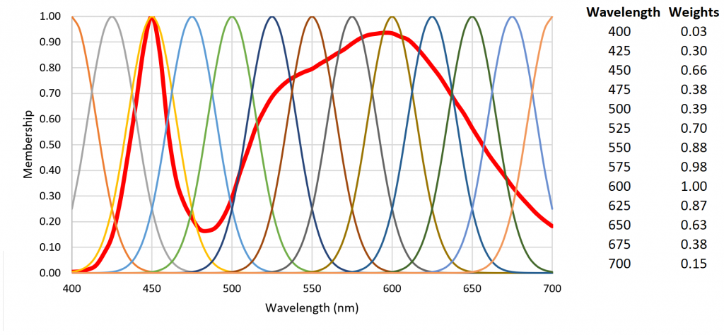
As an example, Figure 7 shows 13 radial basis functions over the visible light range of 400 nm to 700 nm that are each multiplied on a per-wavelength basis by the SPD of a 4000-K white light LED to yield the basis function weights.
Figure 7. Radial basis function weights for a 4000K white LED SPD.
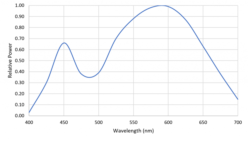
Figure 8 shows a reconstruction of the LED SPD using a cubic spline curve with the weights as knots. The reconstruction is clearly different from the original SPD, but in terms of predicting plant responses, it is likely adequate.
Figure 8. Spline reconstruction of 4000-K white LED SPD from radial basis function weights.
Horticultural Spectral Sensor
Referring to Figure 6, each basis function can be seen as the responsivity of a radiant flux meter in combination with a Gaussian bandpass filter with a center wavelength of xi. Combining the unweighted outputs of the 19 filtered meters results in a flat response from 375 nm to 775 nm. Presented with an arbitrary SPD, the filtered meter outputs represent the appropriate weighting for the basis functions to approximate the SPD. Moreover, the absolute values of the filtered meter outputs can be used to estimate the absolute spectral irradiance incident on the meters, from which can be calculated the absolute irradiance in watts per square meter and the photosynthetic photon flux density (PPFD) in micromoles per square meter per second.
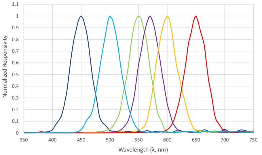
Figure 9 shows the spectral responsivities of an AS7262 6-channel visible light spectral sensor with a spectral range of approximately 430 nm to 570 nm, as manufactured by ams AG of Premstaetten, Austria. While the spectral responsivities are not ideal Gaussian functions, it is clear that an instrument to directly measure radial basis function weights can be fabricated using existing technology.
An advantage of this system and method in terms of horticultural light sources is that the spectral power distributions can be unambiguously measured and expressed as a small set of numbers, regardless of the SPD complexity. If the representations of two SPDs are similar, the horticulturalist may be assured that they will likely have the same biological effect on a plant species. As an example, white light fluorescent lamps typically exhibit a combination of continuum and line spectra, whereas white light LEDs typically exhibit a narrow peak emission near 450 nm and a broad continuum from the blends of green- and red-emitting phosphors (e.g., Figure 7). Regardless, if their sets of radial basis function weights are similar, the two light sources may also be regarded as similar with respect to horticultural applications.
Fuzzy Logic SPD Classifier
The unanswered question is, what does “similar” mean in the context of comparing two or more SPD representations? With 13 to 19 radial basis function weights as parameters, it becomes impractical to formulate a table of rules for comparison purposes. The solution to this problem is a fuzzy logic classifier.
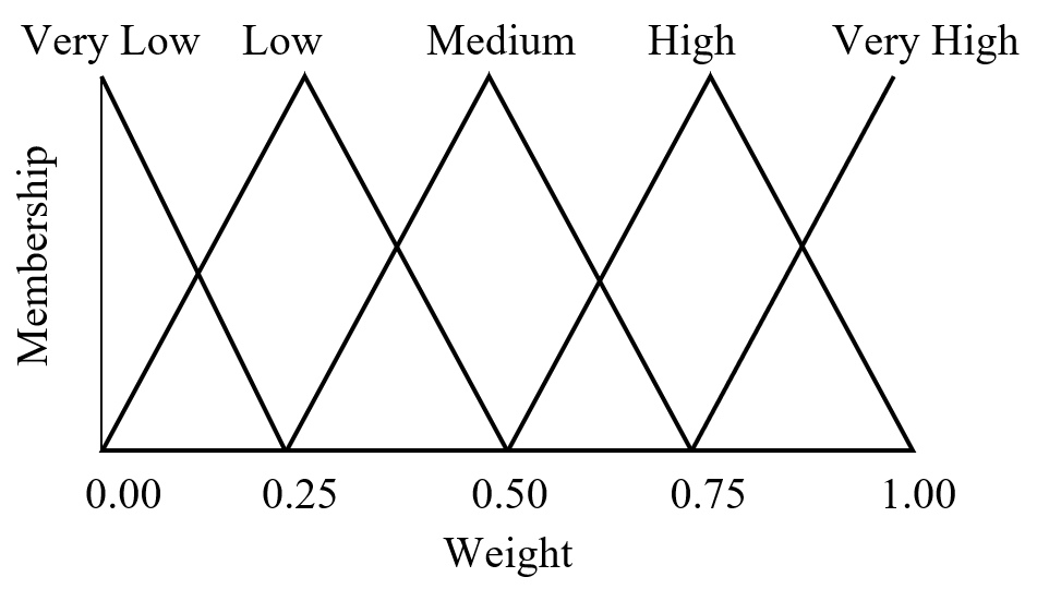
Fuzzy logic is often seen as a mathematical means of representing vagueness and imprecise information when making decisions, where input signals are “fuzzified” by mapping their precise values to a set of fuzzy membership functions. Referring to Figure 10 as an example, a radial basis function with weight 0.85 has membership 0.60 in “high” and membership 0.40 in “very high.” (Triangular membership functions are used in this example, but trapezoidal and sigmoid functions may also be used.)
Figure 10. Fuzzy set with five triangular membership functions.
Referring to Figure 7, the fuzzification of the set of 13 radial basis function weights results in Table 2.
Table 2 – Fuzzification of 4000-K White Light LED SPD
Wavelength
Weight
Very Low
Low
Medium
High
Very High
400
0.03
0.88
0.12
0.00
0.00
0.00
425
0.30
0.00
0.80
0.20
0.00
0.00
450
0.66
0.00
0.00
0.36
0.64
0.00
475
0.38
0.00
0.48
0.52
0.00
0.00
500
0.39
0.00
0.44
0.56
0.00
0.00
525
0.70
0.00
0.00
0.20
0.80
0.00
550
0.88
0.00
0.00
0.00
0.48
0.52
575
0.98
0.00
0.00
0.00
0.08
0.92
600
1.00
0.00
0.00
0.00
0.00
1.00
625
0.87
0.00
0.00
0.00
0.52
0.48
650
0.63
0.00
0.48
0.52
0.00
0.00
675
0.38
0.48
0.52
0.00
0.00
0.00
700
0.15
0.40
0.60
0.00
0.00
0.00
Table 2 – Fuzzification of 4000K white light LED SPD.
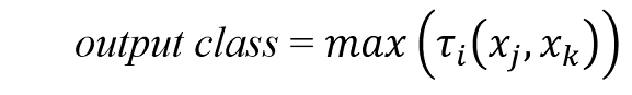
The set of n fuzzified weights for a given SPD is then submitted to a fuzzy if-then rule system. Given any two fuzzified weights x1 and x2 as inputs, a typical fuzzy rule will be:
where there are multiple output classes.
Each rule calculates a “vote” t that is determined by degree of membership m for each fuzzified weight:
and where the fuzzy AND operator is implemented as the minimum of the two membership values.
Once all of the rules have been processed, their votes are aggregated:
for all votes.
This is arguably the simplest possible implementation of a fuzzy logic classifier. There are other methods for calculating and aggregating votes that are likely better for the purpose, but it is the principle that is of interest. What a fuzzy logic classifier accomplishes is a framework for representing expert knowledge of the effect of similar but different SPDs on plant growth and health, taking into consideration the plant species, plant growth stage, plant environmental conditions, and other parameters. In a sense, the fuzzy if-then rules formalize what is known about plant responses to optical radiation (e.g., Table 1) and classify horticultural luminaire SPDs accordingly.
Summary
While light-emitting diodes have provided botanists with the ability to generate precisely controlled SPDs for their research, the use of colloquial color names in their published papers has made it difficult to interpret and summarize their research results for the horticultural industry. This paper therefore proposes the use of a small number of radial basis functions to represent SPDs for horticultural lighting purposes, based on the observation that the absorption characteristics of photopigments in vivo limits the need for more-detailed SPDs. A proposal for a horticultural spectral sensor that measures radial basis function weights directly is also introduced.
Finally, a fuzzy logic classifier is proposed as a means of representing expert knowledge gained from horticultural research using fuzzy if-then rules, thereby resolving the problem of determining the similarity of two or more SPDs for horticultural lighting purposes.
References
ASABE. 2017. ANSI/ASABE S640 JUL2017, Quantities and Units of Electromagnetic Radiation for Plants (Photosynthetic Organisms). St. Joseph, MI: American Society of Agricultural and Biological Engineers.
Both A-J et al. 2017. Proposed product label for electric lamps used in the plant sciences. Hort Technol. 27(4):544-549.
Buhmann, MD, Jäger J. 2000. On radial basis functions. Acta Numerica. 9:1-38.
Craig DS, Runkle ES. 2013. A moderate to high red to far-red light ratio from light-emitting diodes controls flowering of short-day plants. J Am Soc Horticult Sci. 138(3):167-172.
Kuehni RG. 2003. Color Space and Its Divisions. Hoboken, NJ: John Wiley & Sons.
ISO. 2007. ISO 21348:2007(E). Space Environment (Natural and Artificial – Process for Determining Solar Irradiances. Geneva, Switzerland: ISO.
Johkan M et al. 2012. Effect of green light wavelength and intensity on photomorphogenesis and photosynthesis in Lactuca sativa. Environ Exper Botany. 75:128-133.
Maloney L. 1986. Evaluation of linear models of surface spectral reflectance with small number of parameters. J Opt Soc Am. 3(10):1673-1683.
McCree KJ. 1972. The action spectrum, absorptance and quantum yield of photosynthesis in crop plants. Agric Meteorology. 9:191-216.
Moss RA, Lewis WE. 1952. Absorption spectra of leaves. I. The visible spectrum. Plant Physiol. 27(2):370-391.
Sager JC et al. 1988. Photosynthetic efficiency and phytochrome equilibria determination using spectral data. Trans ASABE. 31(5):1882-1889.
Terashima I et al. 2009. Green light drives leaf photosynthesis more efficiently than red light in strong white light: Revisiting the enigmatic question of why leaves are green. Plant Cell Physiol. 50(4):684-697.
Westland S et al. 2000. Colour statistics of natural and man-made surfaces. Sensor Rev. 20(1):50-55.
Westland S, Ripamonti C. 2004. Computational Color Science Using Matlab, Chapter 10. Chichester, UK: John Wiley & Sons.
This website uses cookies (mostly chocolate chip) to improve your experience. We'll assume you're ok with this, but you can opt-out if you wish. Cookie settingsACCEPT
Cookies Policy
Privacy Overview
This website uses cookies to improve your experience while you navigate through the website. Out of these cookies, the cookies that are categorized as necessary are stored on your browser as they are essential for the working of basic functionalities of the website. We also use third-party cookies that help us analyze and understand how you use this website. These cookies will be stored in your browser only with your consent. You also have the option to opt-out of these cookies. But opting out of some of these cookies may have an effect on your browsing experience.
Necessary cookies are absolutely essential for the website to function properly. This category only includes cookies that ensures basic functionalities and security features of the website. These cookies do not store any personal information.
Any cookies that may not be particularly necessary for the website to function and is used specifically to collect user personal data via analytics, ads, other embedded contents are termed as non-necessary cookies. It is mandatory to procure user consent prior to running these cookies on your website.