This is a preprint of a paper presented by the author at the International Society for Horticultural Lighting (ISHS)’s GreenSys 2019 conference in Angers, France in June 2019, and scheduled for publication in Acta Horticulturae .
Abstract
Recent advances in LED-based luminaire design have enabled greenhouse operators to temporally control both the photon flux density (PFD) and spectral irradiance incident upon the plant canopy. However, it is difficult to predict the performance and benefits of these luminaires without knowledge of the time-varying PFD and spectral irradiance due to daylight. We have addressed this problem with the development of horticultural lighting design software that incorporates validated climate-based annual daylighting calculations, physically-based modelling of glazing and light diffusion materials, modelling of spectral reflectance from greenhouse crops and surrounding surfaces, and accurate simulation of optical radiation distribution within the greenhouses from direct sunlight, diffuse daylight, and supplemental electric light sources. These measurements can be used to determine daylight availability, monthly Daily Light Integrals, automated shade and energy curtain deployment schedules, and projected electrical energy costs, all in advance of building the physical structures.
Introduction
Since their commercial introduction in 1964, high-pressure sodium (HPS) lamps have been a mainstay of supplemental electric lighting in greenhouses. With their fixed light outputs and spectral power distributions (SPDs), however, there has been little incentive or opportunity for commercial greenhouse operators with experiment with different “light recipes” for optimum plant growth and health. Rather, the luminaires are typically turned on at dusk and operated until the desired Daily Light Integral (DLI) for the crop or ornamental plats is achieved.
The introduction of light-emitting diodes (LEDs) for horticultural lighting has completely changed this situation. Many luminaire manufacturers are now offering products with separate SPD settings for promoting vegetative growth and blooming. Some manufacturers are going further by including, in addition to the ubiquitous 450 nm blue and 660 nm red LEDs, ultraviolet-A, green and “white light” LEDs with different correlated color temperatures (CCTs), and also 735 nm far-red LEDs. Going further still, a few products can be dimmed in response to inputs from daylight sensors, and it likely that future products will enable computer control of their SPDs beyond simple “veg” and “bloom” settings.
Together, these studies indicate that successful light recipes may involve daily dynamic changes in both the photon flux density (PFD) and SPDs delivered to crops and ornamentals in greenhouses. However, there is a problem. Most of these studies have been conducted in controlled environment growth chambers. It is often difficult to translate such laboratory research to greenhouse environments (e.g., Annunziata et al., 2017). Even if light recipes for a given crop or ornamental are developed in a research greenhouse, it is difficult to ensure that all of the requirements are met in commercial greenhouses. Certainly, such simple metrics as DLI are not enough.
GREENHOUSE MODELLING
Modelling a greenhouse begins with its most important element: glazing.
Glazing
For the purposes of daylighting, glazing materials have three important optical properties:
Fresnel transmittance.
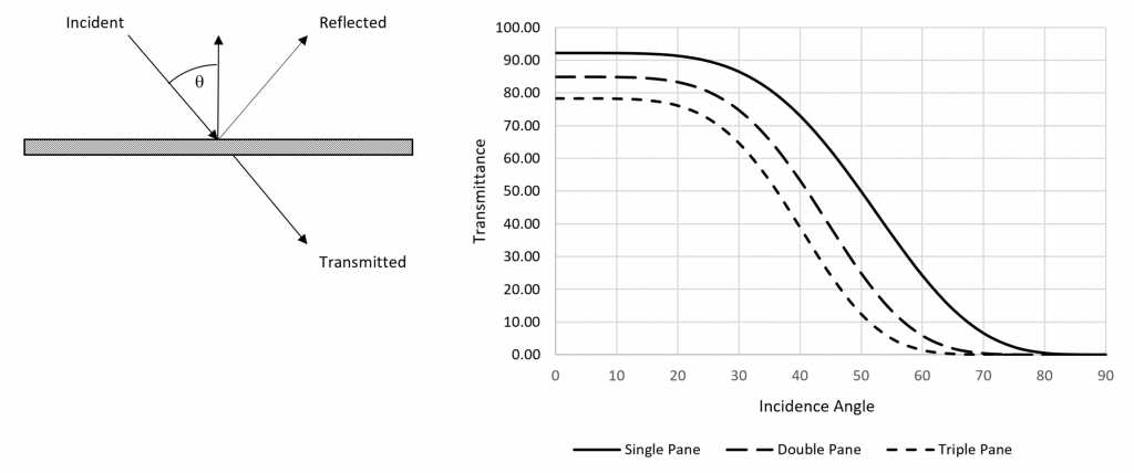
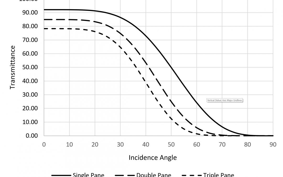
The optical transmittance of transparent glass and rigid plastic panels (collectively dielectric materials) depends on the angle of incidence q of the incoming light (Figure 1). At normal incidence (i.e., q = 0 degrees), each surface reflects about 4 percent of the light. A single pane has two surfaces, and so the maximum possible transmittance is 92 percent. Double-pane and triple-pane insulated glass panels correspondingly have maximum possible transmittances of 85 percent and 78 percent respectively
What is more important is that the transmittance decreases with increasing angle of incidence, as determined by the “Fresnel equations” (e.g., Ashdown, 2019). This is clearly evident when reflections of the Sun from windows are viewed at grazing angles. Anti-reflection (AR) coatings can improve the transmittance somewhat at normal incidence, but the Fresnel transmittance still dominates at large incidence angles.
Figure 1. The transmittance of transparent glazing depends on the angle of incidence q and the number of panes.
It is also important to note that Figure 1 applies to daylight with a specific angle of incidence. Looking at the graph, it is evident that the transmittance of direct sunlight through the greenhouse glazing panels will depend on the solar position (azimuth and altitude), the building orientation, and the roof panel slope. The solar position varies throughout the day and year, of course, and so any transmittance calculations need to be performed on an hourly basis.
What is less evident is that daylight is comprised of both direct sunlight and diffuse daylight. On a clear summer day at noon, the ratio of direct sunlight to diffuse daylight incident on a surface facing the sun may be 20:1 or so; on an overcast day, there is no direct sunlight. In addition, the amount of daylight diffusely reflected from the ground and incident on vertical surfaces is typically 20 percent or so. The graph shown in Figure 1 is therefore instructive but not useful for calculation purposes.
Diffusion.
There is growing evidence that plants use diffuse light more effectively than direct sunlight (e.g., Li and Yang, 2015). Particularly for shade-tolerant plants, translucent glazing results in more even spatial distribution of photosynthetic photon flux (PPFD) within the greenhouse, and also reduces its temporal variation on clear days.
Of course, the analytic modelling method for diffusion materials can also be used to represent greenhouse shade cloth, paint materials, and condensation on otherwise non-diffusing glazing.
Spectral transmittance.
The spectral range of photobiologically active radiation (PBAR) is generally assumed to be 280 nm to 800 nm (ASABE, 2017). This includes ultraviolet-B (280 nm to 315 nm) and ultraviolet-A (315 nm to 400 nm). However, soda-lime glass is opaque to ultraviolet radiation below approximately 320 nm, and so UV-B radiation, while shown to be beneficial to field-grown plants, is not a consideration in greenhouses. Similarly, low-density polyethylene (LDPE) used as an agricultural film for polytunnels, is opaque below 350 nm (Cadena and Acosta, 2014), while polycarbonate is opaque below 390 nm.
Given this, it is reasonable to model spectral irradiance inside greenhouses and polytunnels from 350 nm to 800 nm, where the spectral transmittance of soda-lime glass, LDPE, and polycarbonate is basically constant.
Greenhouse Structure
For most greenhouse designs, the purpose of the greenhouse structure is to support the glazing and possibly fan housings and motorized shades. From the perspective of climate-based daylight modelling, it is the size, position, and orientation of the glazing panels (or film for polytunnels) that is most important.
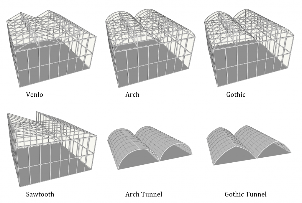
While there are many custom greenhouse designs, almost all commercial greenhouses can be classified as having arch, Gothic, Venlo, or sawtooth roofs, while polytunnels can be classified as having either arch or Gothic hoops (Figure 2).
Gothic Tunnel
Figure 2. Four different greenhouse roof styles and two different polytunnel hoop styles determine how direct sunlight and diffuse daylight are transmitted through the roof panels.
While not directly related to daylight modelling, it would clearly be a time-consuming exercise for a typical user (for example, a greenhouse or horticultural luminaire manufacturer) to design and model an entire greenhouse with all the side posts, rafters, support columns, purlins, and cross ties. Fortunately, the simplicity of the framework makes it possible to use parametric design techniques, where the software generates the entire greenhouse structure from a few user-specified parameters. This can include the dimensions and spacing of tables, the placement of horticultural luminaires as supplemental electric lighting, and the specification of motorized shades.
A computer-aided drafting (CAD) model as shown in Figure 3 and needed for the daylighting calculations can be generated from the user-specified parameters in a fraction of a second. Due to the modular nature of greenhouses, even greenhouses as large as hundreds of thousands of square meters can be generated in the same amount of time.
Figure 3. Automatically-generated CAD model of a Venlo greenhouse.
Horticultural Luminaires
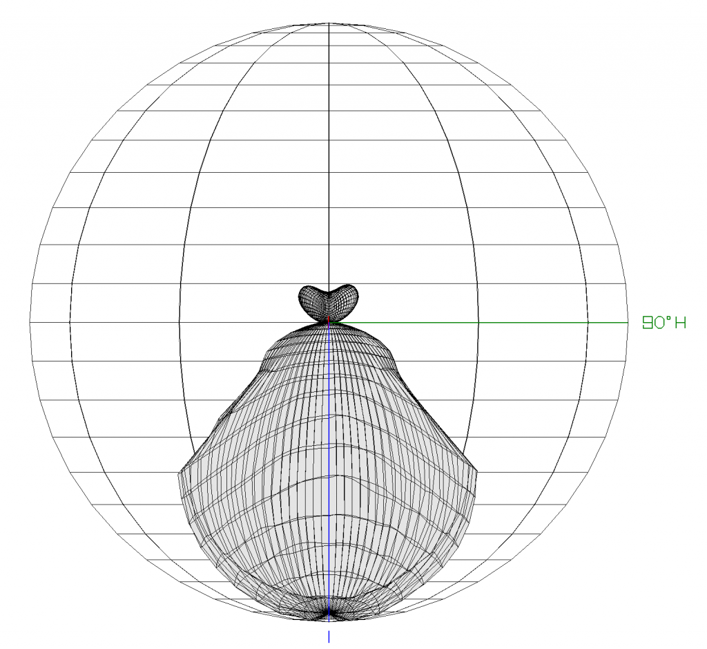
For over a century, architectural luminaires have been modeled as point light sources with angular luminous intensity distributions (Figure 4). For more than thirty years, the laboratory measurements have been reported using formatted text files that lighting design software programs can read.
To address this issue, an international standard was developed with specific support for horticultural lighting. Currently published in the United States (IES, 2018) and Italy (UNI, 2019), it is being developed for publication as a worldwide ISO standard. Its features include:
Photon intensity distribution (measured in µmol ´ sr-1 ´ sec-1)
Total photon flux (measured in µmol ´ sec-1)
Spectral power distribution (measured in watts ´ nm-1)
Channel multiplier
If the luminaire allows the LED color intensities to be individually controlled, these can be represented by a “channel multiplier” for each color that represents the channel dimmer setting when the luminaire’s optical characteristics were measured.
Horticultural luminaire manufacturers currently report photosynthetic photon intensity distributions (or a multiplier to convert from lumens to photon flux). However, future light recipes will require more information than this. Accordingly, the spectral range is specified for the photon measurements (minimum and maximum wavelengths) so that it is possible to represent ultraviolet (280 nm – 400 nm), photosynthetic (400 nm – 700 nm), and far-red (700 nm – 800 nm) photon intensity and flux values (ASABE, 2017).
Weather Data
To calculate the daylight incident on a greenhouse, the software needs to know the building’s latitude, longitude, and compass (orientation). With this, it is possible to locate the nearest weather station for which a Typical Meteorological Year (TMY) weather dataset is available. One example is the collection of EnergyPlus TMY3 datasets, representing over 2,500 locations worldwide, although there are other datasets available that have been derived from combinations of historical weather data and weather satellite observations.
Virtual PAR Sensors
To measure the spatial distribution of PPFD on the plant canopy in the greenhouse, it is necessary to specify a horizontal array of virtual PAR (quantum) sensors. Each sensor will then receive direct sunlight, diffuse daylight, and direct photon flux from the luminaires (if any).
There are no restrictions on the position and orientation of the PAR sensors, so they could also for example be placed between the plant rows and oriented to measure vertical rather than horizontal photon flux, including that reflected from the floor and plant leaves.
Daylight Calculations
Once the greenhouse has been modeled and a weather dataset appropriate for the location obtained, the climate-based annual daylight calculations can be performed. Each weather dataset typically has 8,760 hourly records, so there are 4,380 different daylighting scenarios that must be considered.
The daylight calculations occur in two phases. In the first phase, the daylight incident on the exterior of the building is determined. This includes determining:
The solar position (altitude and azimuth) for a given time and date;
The direct solar irradiance;
The spatial distribution of diffuse daylight radiance on the sky dome;
The daylight diffusely reflected from the ground; and
The daylight SPD.
where the spatial distribution of the diffuse daylight is calculated in accordance with the industry-standard Perez sky model (Perez et al., 1993). The daylight calculation algorithms are detailed elsewhere (Ashdown, 2017).
Daylight SPD
Both direct sunlight and diffuse daylight have SPDs that closely resemble that of a black-body radiator, and so they can be uniquely described by their color temperature, expressed in kelvins (K). Direct sunlight has a color temperature of approximately 5500K, while that of clear blue sky typically ranges from approximately 7500K to 15,000K.
The SPD of daylight with color temperatures greater than 4000K can be calculated using the equations presented in CIE 15:4, Colorimetry (CIE, 2004). For example, the combination of direct sunlight and diffuse daylight on a clear day has a color temperature of approximately 6500K (which is the same white color as a computer display); the corresponding SPD is shown in Figure 6.
For overcast skies, clouds are spectrally neutral and so scatter daylight without changing its SPD. Consequently, a typical overcast sky has a color temperature between 6000K and 6600K (Lee and Hernández-Andréz, 2006). Given this, it is reasonable to assume a color temperature of 5500K for direct sunlight, 10,000K for clear blue sky, and 6500K for overcast sky.
Radiosity calculations
The second phase of the daylight and electric lighting calculations determine the spatial distribution and temporal changes in PPFD within the greenhouse. These calculations use a version of radiative flux transfer equations referred to as the radiosity method, and have been detailed elsewhere (e.g., Ashdown, 1994). Of significance for horticultural lighting design is that even though some 4,380 hourly daylight scenarios must be calculated, the calculation times are on the order of a few seconds to a few minutes, depending on the size of the greenhouse (Ashdown, 2018a).
Automated Shades
Automated shades are a common approach to limit the amount of direct sunlight incident upon the plant canopy. Given this, designated glazing panels in the greenhouse models can be modelled as being both transparent and diffusing (or, for energy curtains, opaque). This has no effect on the daylight or electric lighting calculation times, but it does mean that after the calculations have been completed, the spatial distribution of PPFD within the greenhouse can be accessed on a per-hour basis afterwards with the shades either open or closed.
Virtual Spectroradiometer
Architectural lighting design software models light sources as being “white,” and all surface colors as being combinations of red, green, and blue components. This works well for both lighting calculations and architectural visualizations, but it means that the daylight and luminaire SPDs cannot be represented. (They could, but it would require that the spectral reflectance distributions of all surfaces would need to be known, and greatly increasing the calculation times and memory requirements.)
Fortunately, there are mathematical techniques borrowed from remote satellite imaging that obviate the need for spectral reflectance distributions (e.g., Fairman and Brill, 2004). Instead, given only the red, green and blue components of a color, it is possible to reconstruct a physically plausible SPD. With this, it is possible to implement a virtual spectroradiometer that can be positioned and oriented anywhere in the greenhouse after the lighting calculations have been completed.
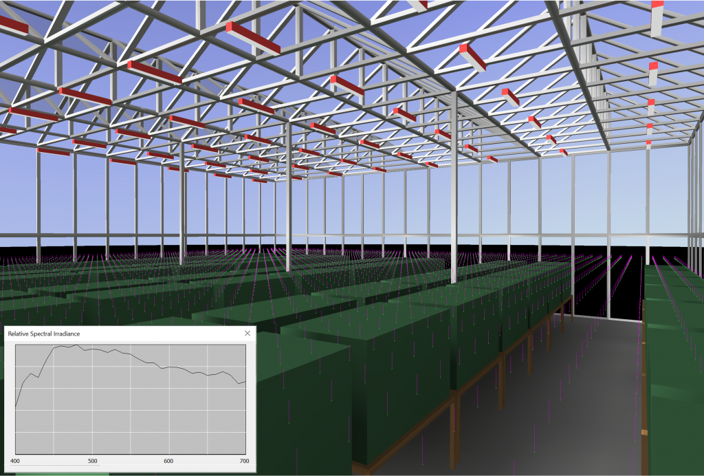
Figure 5. Virtual spectroradiometer measuring daylight SPD inside a greenhouse.
RESULTS ANALYSIS
Once the daylight and electric lighting calculations have been completed, the most obvious analyses include calculating the predicted monthly DLIs and predicted electrical energy costs for the proposed buildings. However, new tools introduce new opportunities, and CBDM for greenhouses is no exception.
As one example, shade fabrics are available with a wide range of absorption and diffusion characteristics. By modelling different fabrics in software, it is possible to determine which will offer the best performance for different crops, taking into account the monthly DLIs and peak PPFDs rather than simply calculating an example time and date.
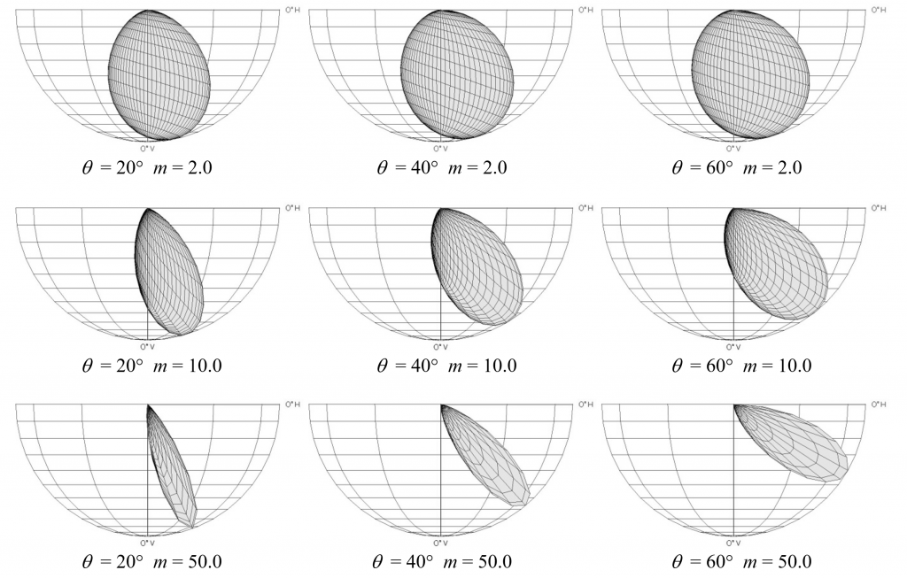
Figure 6. Analytic bidirectional scattering distribution function (BSDF) of diffiuion material.
Automated shades and energy curtains are another example. The calculation results can be used to develop automatic shade deployment schedules in response to changing weather conditions. It may be, for example, that the shades are ineffective – something that can be determined during the design phase rather than after construction.
Yet another example is light pollution. Increasing attention is being paid to the negative aspects of greenhouse lighting at night – light trespass onto neighbouring residential properties, increased sky glow (especially on overcast nights with low cloud cover), and ecological disruption for both animals and plants. Greenhouse lighting design software can be used to model and predict these problems. (As one particular example, roof-mounted energy curtains can potentially result in a 20 percent or more reduction in electrical operating costs due to the light being reflected back down onto the plant canopy.)
Finally, a virtual spectroradiometer is the ideal tool for predicting the spectral distribution of photon flux anywhere in the greenhouse. As light recipes become more sophisticated, such a tool becomes increasingly valuable.
CONCLUSIONS
As stated in the introduction, the goal of this paper has been to report on the development of climate-based daylight modelling software specifically for greenhouses and polytunnels with optional supplemental electric lighting. The focus has been on the horticultural aspects of the software from a user’s perspective, with as few references to computer science and related topics as possible. To do otherwise would have required at least several textbooks worth of material.
The real goal of this paper has been to introduce what is basically a new tool for greenhouse designers, and to explore the issues that it addresses. This paper will hopefully provide the foundation for further conversations between horticulturalists and software developers responsible for such tools.
ACKNOWLEDGEMENTS
The author wishes to thank Peter Socha for his assistance in the research for this paper.
Literature cited
Annunziata, M.G., Apelt, F., Carillo, P., Krause, U., Feil, R., Mengin, V., Lauxmann, M.A., Köhl, K., Nikoloski, Z., Stitt, M., et al. J.E. (2017.) Getting back to nature: a reality check for experiments in controlled environments. J. Exp. Bot. 68 (16), 4463–4477 http://dx.doi.org/10.1093/jxb/erx220.
ASABE. (2017.) ANSI/ASABE S640 JUL2017, Quantities and Units of Electromagnetic Radiation for Plants (Photosynthetic Organisms). (St. Joseph, MI: American Society of Agricultural and Biological Engineers.)
Ashdown, I. (1994.) Radiosity: A Programmer’s Perspective. (New York, NY: John Wiley & Sons.)
Ashdown, I. (2016.) Climate-based daylight modeling: from theory to practice. http://dx.doi.org/10.13140/RG.2.2.19325.20969.
Ashdown, I. (2017.) Analytic BSDF modeling for daylight design. Paper presented at: IES 2017 Annual Conference, Portland, OR. (New York, NY: Illuminating Engineering Society).
Ashdown, I. (2018a.) LICASO and DAYSIM: a comparison. http://dx.doi.org/10.13140/RG.2.2.25669.09441.
Ashdown, I. (2018b.) Far-red lighting and the phytochromes. Maximum Yield 20 (7), 60-66 (October).
Ashdown, I. (2019.) Light transmittance through greenhouse glazing. Maximum Yield 21 (3), 50-51 (March).
Cadena., C., and Acosta, D. (2014.) Effects of solar UV radiation on materials used in agricultural industry in Salta, Argentina: study and characterization. J. Mat. Sci. Chem. Eng. 2, 1-14 http://dx.doi.org/10.4236/msce.2014.24001.
CIE. (2004.) Colorimetry, Third Edition. CIE Technical Report 15:2004. (Vienna, Austria: Commission Internationale de l’Eclairage.)
Craig, D.S., and Runkle, E.S. (2013.) A moderate to high red to far-red light ratio from light-emitting diodes controls flowering of short-day plants. J. Am. Soc. Hortic. Sci. 138 (3), 167–172 http://dx.doi.org/10.21273/JASHS.138.3.167.
Demotes-Mainard, S., Péron, T., Corot, A., Bertheloot, J., Gourrierec, J., Pelleschi-Travier, S., Crespel, L., Morel, P., Huché-Thélier, L., Boumaza, R., et al. (2016.) Plant responses to red and far-red lights, applications in horticulture. Env. Exp. Bot. 121, 4–21 http://dx.doi.org/10.1016/j.envexpbot.2015.05.010.
Fairman, H.S., and Brill, M.H. (2004.) The Principal Components of Reflectances. Color Res. App. 29 (2), 104-110 http://dx.doi/10.1002/col.10230.
Giancomelli, G.A. (2011.) Greenhouse Glazing. In Ball Redbook Vol. 1., 18th edn, C. Beytes, ed. (Chicago, IL: Ball Publishing), p.23-41.
Hanyu, H., and Shoji, K.. (2002.) Acceleration of growth in spinach by short-term exposure to red and blue light at the beginning and at the end of the daily dark period. Acta Hortic. 580, 145-150 http://dx.doi.org/10.17660/ActaHortic.2002.580.17.
Huché-Thélier, L., Crespel, L., Gourrierec, J., Morel, P., Sakr, S., and Leduc, N. (2016.) Light signaling and plant responses to blue and UV radiations – perspectives for applications in horticulture. Env. Exp. Bot. 121, 22–38 http://dx.doi.org/10.1016/j.envexpbot.2015.06.009.
IES. (2018.) ANSI/IES TM-33-2018, Standard Format for the Electronic Transfer of Luminaire Optical Data. (New Yok, NY: Illuminating Engineering Society.)
Lee, R.L., and Hernández-Andrés, J. (2006.) Colour of the Daytime Overcast Sky. App. Optics 44 (27), 5712-5722 http://dx.doi.org/10.1364/AO.44.005712.
Li, T., and Yang, Q. (2015.) Advantages of diffuse light for horticultural production and perspectives for further research. Front. Plant Sci. http://dx.doi.org/10.3389/fpls.2015.00704.
Liu, H., Fu, Y., Hu, D., Yu, J. and Liu, H. (2018.) Effect of green, yellow and purple radiation on biomass, photosynthesis, morphology and soluble sugar content of leafy lettuce via spectral wavebands ‘knock out’. Sci. Hortic. 236, 10–17 http://dx.doi.org/10.1016/j.scienta.2018.03.027.
Perez, R., Seals, R., and Michalsky, J. (1993.) All-weather model for sky luminance distribution – preliminary configuration and validation. Solar Energy 50 (3), 235-245. http:///dx.doi.org/10.1016.0038-092X(93)90017-I.
Ponce, P., Molina, A., Cepeda, P., Lugo, E, and MacCleery, B.. (2015.) Greenhouse Design and Control. (Leiden, The Netherlands: CRC Press/Balkema.)
Seaton D.D., Toledo-Ortiz, G., Ganpudi, A., Kubota, A, Imaizumi, T., and Halliday, K.J. (2018.) Dawn and photoperiod sensing by phytochrome A,”. PNAS 115 (4), 10523–10528 http://dx.doi.org/10.1073/pnas.1803398115.
Song, Y.H., Kubota, A., Kwon, M.S., Covington, M.F., Lee, N., Taagen, E.R., Cintrón, D.L., Hwang, D.Y., Akiyama, R., Hodge, S.K., et al. (2018.) Molecular basis of flowering under natural long-day conditions in Arabidopsis. Nature Plants 4, 824-835 http://dx.doi.org/10.1038/s41477-018-0253-3.
Tregenza, P., and M. Wilson. (2015.) Daylighting: Architecture and Lighting Design. (London, UK: Routledge.)
UNI. (2019. UNI 11733:2019, Luce e illuminazione – specifiche per un formato di interscambio dati fotometrici e spettrometrici degli apparecchi di illuminazione e delle lampade. store.uni.com.
Verdaguer, D., Jansen, M.A.K., Llorens, L., Morales, L.O., and Neugart, S.. (2017.) UV-A radiation effects on higher plants: exploring the known unknown. Plant Sci. 255, 72–81 http://dx.doi.org/10.1016/j.plantsci.2016.11.014.
Wang, Y., and Folta, K.M. (2013.) Contributions of green light to plant growth and development. Am. J. Bot. 100 (1), 70–78 http://dx.doi.org/10.3732/ajb.1200354.
Wargent, J.J., Nelson, B.W.C., McGhie, T.K., and Barnes, P.W. (2015.) Acclimation to UV-B radiation and visible light in Lactuca sativa involves up-regulation of photosynthetic performance and orchestration of metabolome-wide responses. Plant, Cell Env. 38 (5), 929–940 http://dx.doi.org/10.1111/pce.12392.
Wargent, J.J. (2016.) UV LEDs in horticulture: from biology to application. Acta Hortic. 1134, 25–32 http://dx.doi.org/10.17660/ActaHortic.2016.1134.4.
Supplemental electric lighting for greenhouses may be essential for extending the growing season in northern climates, but it comes with a not-so-hidden cost: environmental light pollution. The consequences of this pollution may range from irate neighbours in rural areas to municipal bylaws that may prohibit the use of supplemental lighting during certain hours of the night or altogether.
Searching for information on light pollution online will yield plenty of results. However, it soon becomes apparent that it does not apply to greenhouse lighting. Most of the discussion concerns astronomical light pollution, which is of interest to both amateur and professional astronomers, and where the focus is on outdoor lighting for roadways and parking lots. There are also discussions of “light trespass” onto residential properties from adjacent street lighting, which is rarely a concern for commercial greenhouses.
In addition, there are discussions of the effects of “artificial light at night” (ALAN) on nocturnal wildlife, including insects, fish, amphibians, and mammals. This is a complicated topic, as the effects differ between species and genera. There is almost nothing, however, that is specific to supplemental lighting for commercial greenhouses.
This can be a problem, particularly if citizen action committees lobby government agencies for bylaws and regulations. While alleviating light pollution is a laudable goal, it is necessary for all sides – concerned citizens, municipal authorities, and commercial greenhouse operators – to know the facts and discuss the matter accordingly. Beyond this, there needs to be agreement on what can reasonably be done to alleviate any problems.
At present, the primary source of information for citizen groups are publications from the International Dark-Sky Association (www.darksky.org) in North America and allied organizations in Europe (e.g., www.savethenight.eu). In Canada, the Royal Astronomical Society of Canada has its Light Pollution Abatement Program (www.rasc.ca/lpa) with similar goals. The goal of this article is therefore to look at light pollution in the context of greenhouse supplemental lighting.
Astronomical Light Pollution
Concerns over light pollution began in the 1950s, when the light from large cities began to interfere with astronomical observations made from nearby observatories. (The Dominion Astrophysical Observatory, for example, is only 10 km away from downtown Victoria, BC.) A combination of urban and suburban growth, coupled with the changes from incandescent street lamps to more efficient (and much brighter) mercury vapour and later high-pressure sodium (HPS) lamps, continually exacerbated the problem.
The problem is that even on a clear night, light emitted by roadway and parking lot light fixtures (aka “luminaires”) is reflected from the ground into the night sky. While most of this light escapes into outer space (as we can clearly see when flying over cities at night), a small but significant portion is backscattered down towards the ground by air molecules and airborne dust and smog. The resultant “sky glow” obscures our view of the fainter stars (particularly the iconic Milky Way), and of course interferes with observations by both professional and amateur astronomers.
By itself, a single roadway luminaire does not contribute significantly to sky glow; it is the cumulative effect of thousands to tens of thousands of luminaires in a city that is the problem. Large commercial operations, however, may have thousands of horticultural luminaires and so be equivalent to a small city in terms of light pollution. (Hybrid greenhouses for cannabis production, for example, may have as many as eight hundred 1,000-watt HPS luminaires per acre.)
Spectral Issues
In rural areas away from city smog, the relative amount of backscattered light from roadway luminaires is dependent on the spectral power distribution (or more colloquially, “spectrum”) of the light source. In particular, air molecules (primary nitrogen and oxygen) scatter blue light more effectively than red light (which is why the sky appears blue to us).
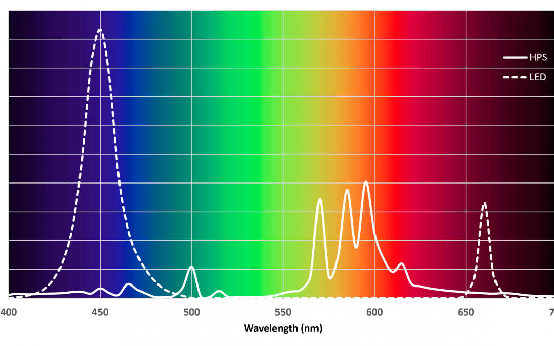
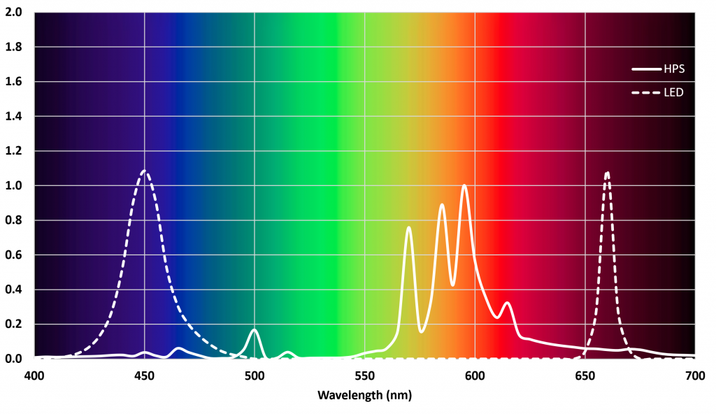
Figure 1 shows the spectra of typical high-pressure sodium (HPS) and light-emitting diode (LED) lights used for greenhouse supplemental lighting. The HPS luminaires look yellow-orange to us, while the LED luminaires appear, depending on the ratio of red to blue light (between 1:1 for vegetative growth to 6:1 for reproductive growth), as various shades of purple (or “blurple”). Figure 1 assumes a 1:1 ratio, which is the worst-case scenario for light pollution. The spectra have been scaled such that both light sources produce equal amounts of photosynthetically active radiation (PAR).
FIG. 1 – Relative lamp spectra.
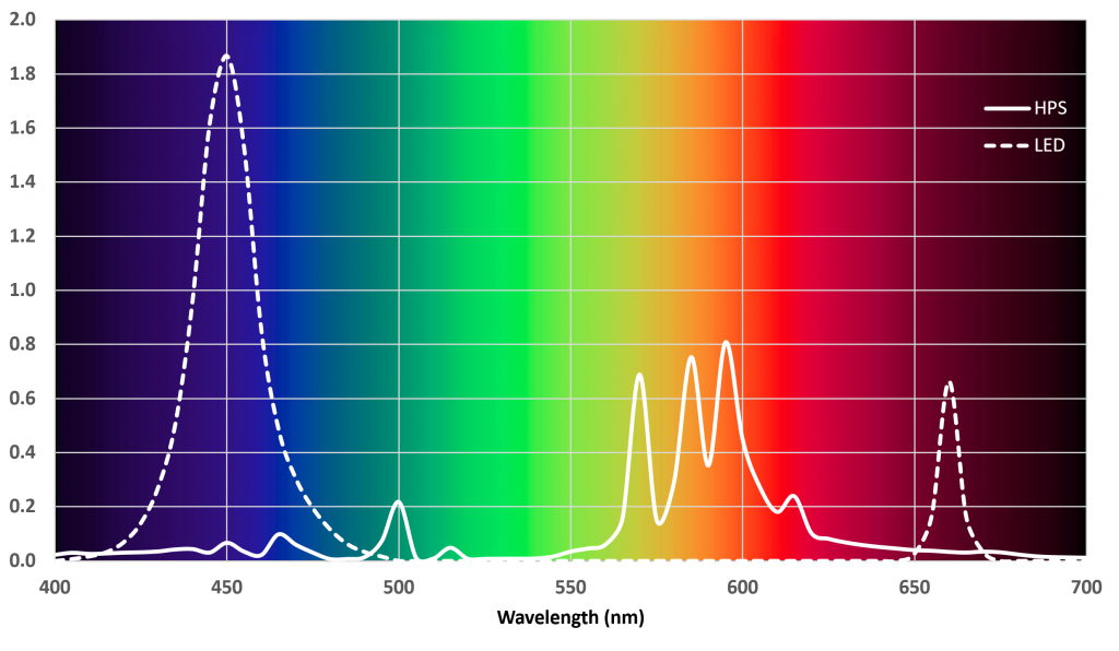
Following IDA and similar publications on astronomical light pollution, concerned citizens and municipal engineers may say something like this: “The amount of backscatter increases as the fourth power of the inverse of wavelength. The blue light of horticultural LEDs will produce much more light pollution than HPS!” This is correct, but it does not explain the situation very well. Figure 2 illustrates what this mean: the amount of backscattered blue LED light is roughly twice that of the backscattered HPS light.
FIG. 2 – Backscatter lamp spectra.
This however does not tell the full story. When our eyes are fully dark-adapted on a starry night, we are most sensitive to blue-green light (actually 505 nm) and less sensitive to yellow and blue. When we take this into account, the increase in astronomical light pollution when changing from HPS to 1:1 blue-red LED lighting is a walloping 3.8 times.
Ecological Light Pollution
Less often talked about but perhaps even more important are the effects of electric lighting on animal and plant life. It is impossible to cover all of these effects here, in part because ecological light pollution is the subject of intense ongoing research by biologists and ecologists. Rodents such as mice are most sensitive to green light and ultraviolet radiation, some migratory birds and bats are most affected by green light, insects respond to ultraviolet radiation, and plants can be impacted by red and far-red light, which disrupts their growth and development. Mammals, reptiles, amphibians, birds, insects … perhaps the best that can be said is that any excess light at night can be considered ecological light pollution, regardless of its spectrum.
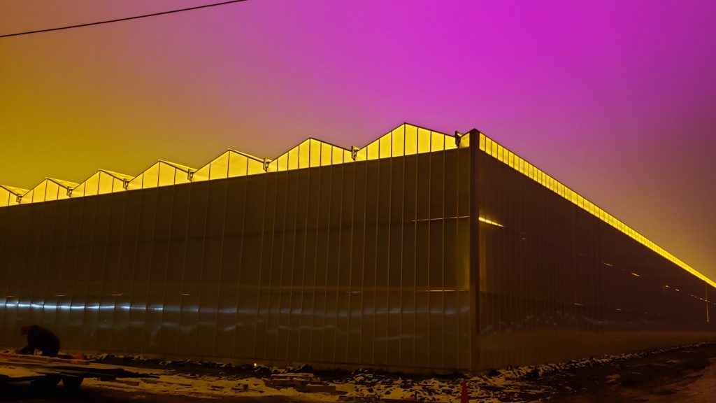
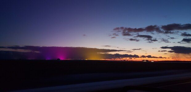
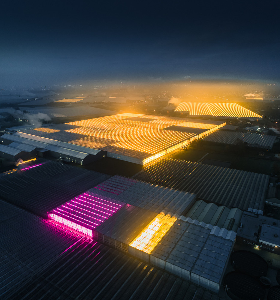
While little research has been devoted to the topic to date, there is also the question of whether light pollution from greenhouses (FIG. 3 and FIG. 4) adversely impact birds, bats, and insects. In urban areas, tens of million migratory birds die every year from nighttime collisions with office tower windows. The US Fish and Wildlife Service is more specific – an estimated 6.6 million migratory birds die each year from collisions with communication towers and their warning lights. While migratory animals may not die from collisions with greenhouses, they are likely disoriented by the bright lights and may suffer increased mortality rates due to exhaustion.
FIG. 3 – Greenhouse light pollution near Leamington, ON. (Source: Detroit News)FIG. 4 – Green house light pollution near Kingsville, ON. (Source: CBS News / Peter Loewen)
Cloudy Nights
Concerned citizens may lobby their municipal councils to “take back the night” so that their children can experience the starry nights they may remember as children, but little attention is paid to overcast nights, when the light pollution can be much worse.
On a clear night, the amount of backscattered light is miniscule – we only notice it because the night sky without light pollution can be exceedingly dark. Low-level stratus clouds, in the other hand, can reflect up to 75 percent of the light reflected from the ground.
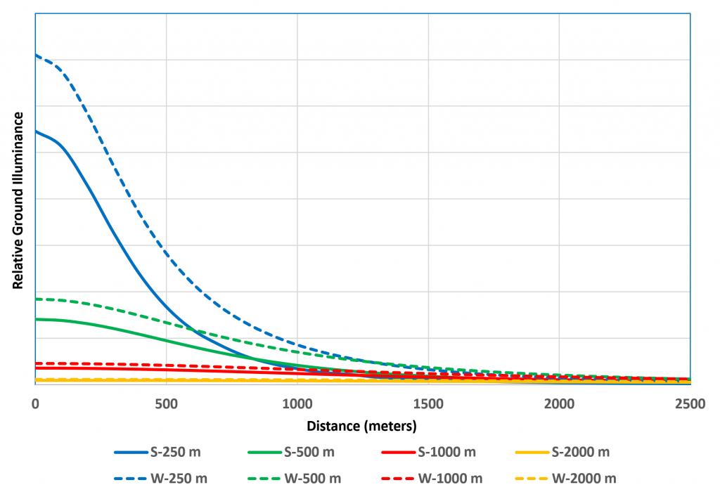
For greenhouses, it all depends on the cloud ceiling height (FIG. 4). If it is 2,000 meters, any light from the greenhouse facility reflected from the clouds will be spread over an area of perhaps ten square kilometers and be reasonably unobtrusive. However, if the ceiling height is 250 meters, the area within a radius about 1500 meters will receive up to 60 times the amount of light pollution on the ground. If the greenhouses are near a sensitive ecological area, this can be a problem.
The amount of light pollution on the ground also depends on the average ground reflectance. For most of the year, this is between 5 and 10 percent. During the winter months with snow on the ground, however, it can increase to anywhere from 40 to 90 percent. Figure 5 shows the differences for summer (solid lines) and winter (dashed lines) ground conditions assuming 10 percent and 80 percent ground reflectance respectively.
FIG. 5 – Relative light pollution versus cloud ceiling height.
The visibility of light reflected from the clouds is another matter entirely, as this depends on the cloud opacity and whether the clouds can be seen on the horizon on an otherwise clear night. Brightly illuminated clouds may disorient migratory animals, again possibly increasing mortality rates due to exhaustion. They may also lad to complaints from residents living a considerable distance from the greenhouses.
Solutions
The simplest solution for most light pollution situations is to use the minimum amount of light needed, and turn the luminaires on only when needed. Unfortunately, this is rarely practical for greenhouse operations. Each crop has specific PAR and daily light integral (DLI) requirements. In response to the suggestion that fewer luminaires could be used or the luminaires turned on for fewer hours at night, each crop has specific requirements related to its circadian rhythms. Like animals, plants need to sleep at night. There may be some flexibility in the supplemental lighting schedule, but likely not enough to make a difference.
What will make a difference are blackout curtains on both the walls and roof of the greenhouse that can be closed at night. The name “blackout” notwithstanding, the preferred color facing inwards is white. In a large greenhouse where the floor area is much greater than the wall area, most of the light from the luminaires will be reflected from the plant canopy and ground through the roof panels. If the average floor reflectance is 10 percent and the curtain reflectance is 80 percent, the plant canopy will receive an additional 20 percent of light.
If a white polyethylene ground cover is used for the greenhouse floor, the average floor reflectance (assuming walkways between the plants) will likely be in the range of 40 to 50 percent. The light will in this case bounce back and forth between the floor and ceiling at least ten times before it is essentially absorbed by the plants, curtains, and floor cover. Each bounce provides further PAR for the plant canopy, so that the end result may be over 100 percent of additional light.
Whatever the amount of additional light received by the plant canopy, it is quite literally recycled light. It reduces the need for supplemental lighting, and can be seen as an operating cost offset to the capital and operating cost of the blackout curtains (which can also function as energy curtains in cold climates).
It is also worth noting that this recycled light is diffuse, and is directed at the plant leaves from both above and below. For many greenhouse crops, this can be beneficial, resulting in stronger stems and less leaf senescence.
Being Proactive
In communities with large concentrations of greenhouses, such as Leamington, ON, light pollution is receiving increasing scrutiny from the press. You know you have a problem when the Detroit Press runs a major article on the light pollution from greenhouses located 25 miles away from the city.
LTO Nederland, the Dutch greenhouse industry organization, has been proactive in mandating screening for 98 percent of the greenhouse if lighting is being used during nighttime hours. If the light levels are greater than 15,000 lux during the hours of 5:00 PM to midnight, the screens need to block 98 percent of the light during the entire night, with the side screens blocking a minimum of 95 percent during nighttime hours.
FIG. 6 – Greenhouse light pollution in the Netherlands. Copyright 2019 Tom Hegen (www.tomhegen.de)
If greenhouse operators wait until their municipalities begin discussing regulations and bylaws, it may put them at a considerable disadvantage. With so little information available to municipal engineers and planners to formulate proposed regulations, it may be advisable to be proactive.
Summary
There is no question that supplemental electric lighting in greenhouses can cause significant environmental light pollution. Having facts and figures available when discussing the issue with concerned citizens and municipal authorities is useful; having a solution that may reduce operating costs is a bonus.
In these unfortunate times, it seems that everyone is looking for ways to help with the COVID-19 crisis. From a lighting designer’s perspective, one solution is obvious: ultraviolet radiation. We have known about the disinfectant properties of ultraviolet radiation for nearly 150 years (Downes and Blunt 1877), and we have been using low-pressure mercury arc lamps to kill bacteria and inactivate viruses for the past 85 years (Wells and Fair 1935).
My initial goal in writing this article had been to discuss ultraviolet germicidal irradiation (UVGI) methods and materials, but this work was pre-empted by the Illuminating Engineering Society’s Photobiology Committee and their excellent report, IES CR-2-20-V1, Germicidal Ultraviolet (GUV) – Frequently Asked Questions.
I can highly recommend this publication for any questions related to ultraviolet disinfection and germicidal lamps, as it is written so as to be accessible to both lighting professionals and the general public. However, there is one small but critical omission that needs to be addressed.
Consumer Interests
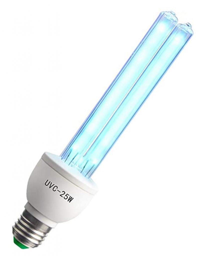
Many consumers are currently interested in ultraviolet sterilizers for home use. Earlier this month, Forbes published an article titled, “Seven of the Best UV Sterilizers for Phones and Other Household Objects.” These devices included a USB UV sanitizer wand, two UV smartphone cleaning cases, a UV water bottle purifier cap, a portable UV sterilizer for small items such as baby pacifiers, an ultraviolet LED sanitization box, and a 25-watt germicidal lamp. Six of these are reasonable and perfectly safe if used correctly. The seventh … well, we need some background to explain the problem.
The ABCs of Ultraviolet
The Commission Internationale de l’Eclairage (CIE) divides the ultraviolet region of the electromagnetic spectrum into three subregions according to wavelength:
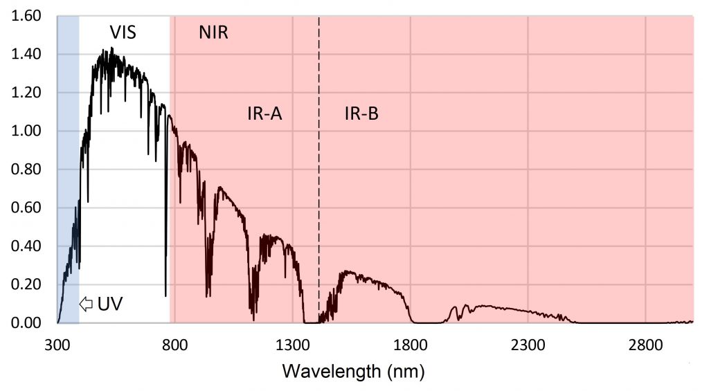
In the natural environment, the only significant source of ultraviolet radiation is sunlight. As the solar spectrum shown in Figure 1 shows, this radiation is only a small fraction of the total radiation received from the Sun. Our atmosphere fortunately absorbs much of the carcinogenic UV-B radiation at sea level, and essentially all of the UV-C radiation, thanks to the Earth’s ozone layer. The risk of exposure to UV-C radiation is therefore entirely from electric light sources.
FIG. 1 – Solar spectrum at sea level.
Now, there are several types of light sources that emit UV-C radiation, but only low-pressure mercury arc lamps and UV-C light-emitting diodes (LEDs) are found in consumer products. We can therefore ignore high-pressure mercury arc lamps, pulsed xenon arc lamps, and krypton-chlorine excimer lamps – this article is about ultraviolet disinfection solution for consumers.
History
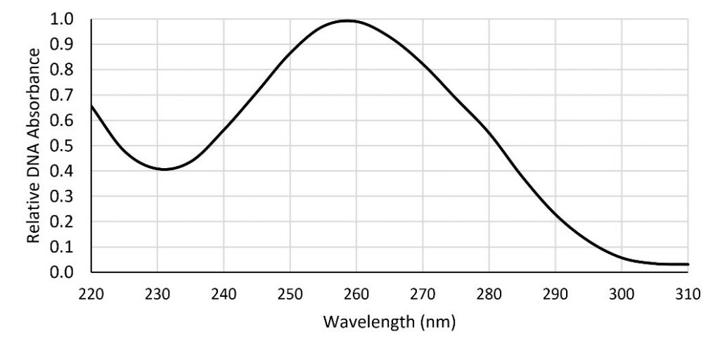
In 1931, F. L. Gates demonstrated that UV-C radiation effectively kills bacteria and protozoa, and inactivates viruses. Using a high-pressure mercury-vapor arc lamp, he produced an “action spectrum” showing effectiveness versus wavelength (Gates 1931). He further noted that this spectrum was very similar to the absorbance spectrum of deoxynucleic acid (DNA), and correctly surmised that the radiation was terminally disrupting the DNA molecules (Figure 2).
FIG. 2 – DNA damage action spectrum (base on E. coli).
The advantage of low-pressure mercury arc lamps is that they emit monochromatic UV-C radiation at 254 nanometers, which is close to the 265 nm peak of Gates’ action spectrum. Even better, these lamps are basically the same as compact and linear fluorescent lamps, but with two important differences: 1) they do not have a phosphor coating to convert the ultraviolet radiation into visible light; and 2) they use fused quartz or soda-lime “soft” glass rather than borosilicate glass for their envelopes. (Fused quartz is transparent at UV-C wavelengths, whereas borosilicate glass is opaque.)
UV-C Exposure Limits
The problem with germicidal lamps is that exposure to UV-C radiation can irritate the eyes and skin. These irritations are technically photokeratitis (“snow blindness” or “welder’s flash”), photoconjunctivitis (“pink eye”), and erythema (sunburn). This medical terminology belies the seriousness of the issue, but a short paper by Trevisan et al. (2006) puts it into perspective.
In 2005, twenty-six medical students attended a 90-minute anatomy lesson in an autopsy room at the University of Padova in Italy. There were three autopsy tables, above each of which was mounted a single 40-watt germicidal lamp. A timer turned the lamps on at 7:00 PM and off at 7:00 AM; the lesson began at 8:30 AM.
Unfortunately for the students involved, the timer failed. They were dressed in protection suits against biological risk, but their eyes and the skin of their faces, scalps and necks were exposed to UV-C radiation for the duration of the lesson. As is common with UV-C exposure, the onset of symptoms occurred on average four hours afterwards. For the eyes, these included a burning sensation, excessive tearing, pain, blurry vision, hindrance to open, conjunctival redness, eyelid swelling, and photophobia. For the skin, the symptoms included acute sunburn, a burning sensation, irritation, and pain. The paper further noted an ocular “foreign body sensation,” which translates into a feeling of having sand constantly in your eyes. These problems lasted two to four days, but six students afterwards reported persistent scurf (flaking of the skin), and one of persistent dryness of the skin.
There are two important points here: 1) the lamps were basically 40-watt linear fluorescent lamps; and 2) the exposure time was only 90 minutes. The horizontal irradiance was later measured and found to vary between 50 μW/cm2 at the level of the autopsy table to 250 μW/cm2 one meter below the germicidal lamps. To put this into perspective, a horizontal illuminance of 500 lux is equivalent to approximately 250 μW/cm2 of visible light.
The American Conference of Governmental Industrial Hygienists recommends a maximum UV-C exposure dose limit for a workday of 3.0 millijoules per square centimeter (ACGIH 2020). For a period of 90 minutes, this translates into an effective irradiance of 0.6 μW/cm2. The students exceeded this recommendation by a factor of 100 to 400 times.
UV-C at Home
You might dismiss the misfortune of the medical students as an unfortunate workplace accident. After all, who would want to have a high-power germicidal lamp in their home?
… which brings us to the seventh UV sterilizer listed in the Forbes article:
The description of this lamp reads, “UV Germicidal Bulb 25w E26/E27 Screw Socket UV Light Bulb 110 Volt, UVC Ozone Free.” It was priced at $35 on 2020/04/02, but is currently (two weeks later) priced at $75. It is clearly a product that is in demand, although the description is less than reassuring:
“When this bulb lit, will immediately have a special smell in the air, it means it worked, this special smell comes from burnt harmful smalls by the UVC ray, just like the smell in the hospital.”
Th manufacturer explicitly states that this product has a quartz envelope and emits 253.7 nm UV-C radiation, but … 25 watts? Considering the medical distress that the medical students suffered from 40-watt lamps, surely this is incorrect?
Apparently not, for the manufacturer also claims that it will sanitize up to 400 square feet (37 square meters) in 15 to 60 minutes, making it “suitable for basement, bathroom, school, canteen, kindergarten, home, salon, closet, hotel … shoe cabinet, dog/chicken house, toilet …” and so on. The Forbes reviewer helpfully added that, “This UV bulb can be screwed into any standard light socket in your home or office.”
Nowhere on the Amazon Web page is there any mention as to how dangerous the output from a 25-watt germicidal lamp can be. “Wait,” you say, “surely this product has to comply with the relevant government regulations designed to protect consumers from such unseen dangers?”
If you are an American, the Occupational Safety and Health Administration has this to say as a standards interpretation: “… there are no OSHA-mandated employee exposure limits to ultraviolet radiation.” If you are a Canadian, the Canadian Center for Occupational Health and Safety says, “There are no Canadian regulatory occupational exposure limits for UV radiation. Many jurisdictions follow the limits recommended by the American Conference of Governmental Industrial Hygienists (ACGIH).”
There are government standards regulating the emission of UV-B radiation from suntanning beds and ultraviolet emissions from white-light mercury vapor lamps … but apparently nothing for UV-C disinfectant lamps. In other words, dear consumer, caveat emptor.
Wild West
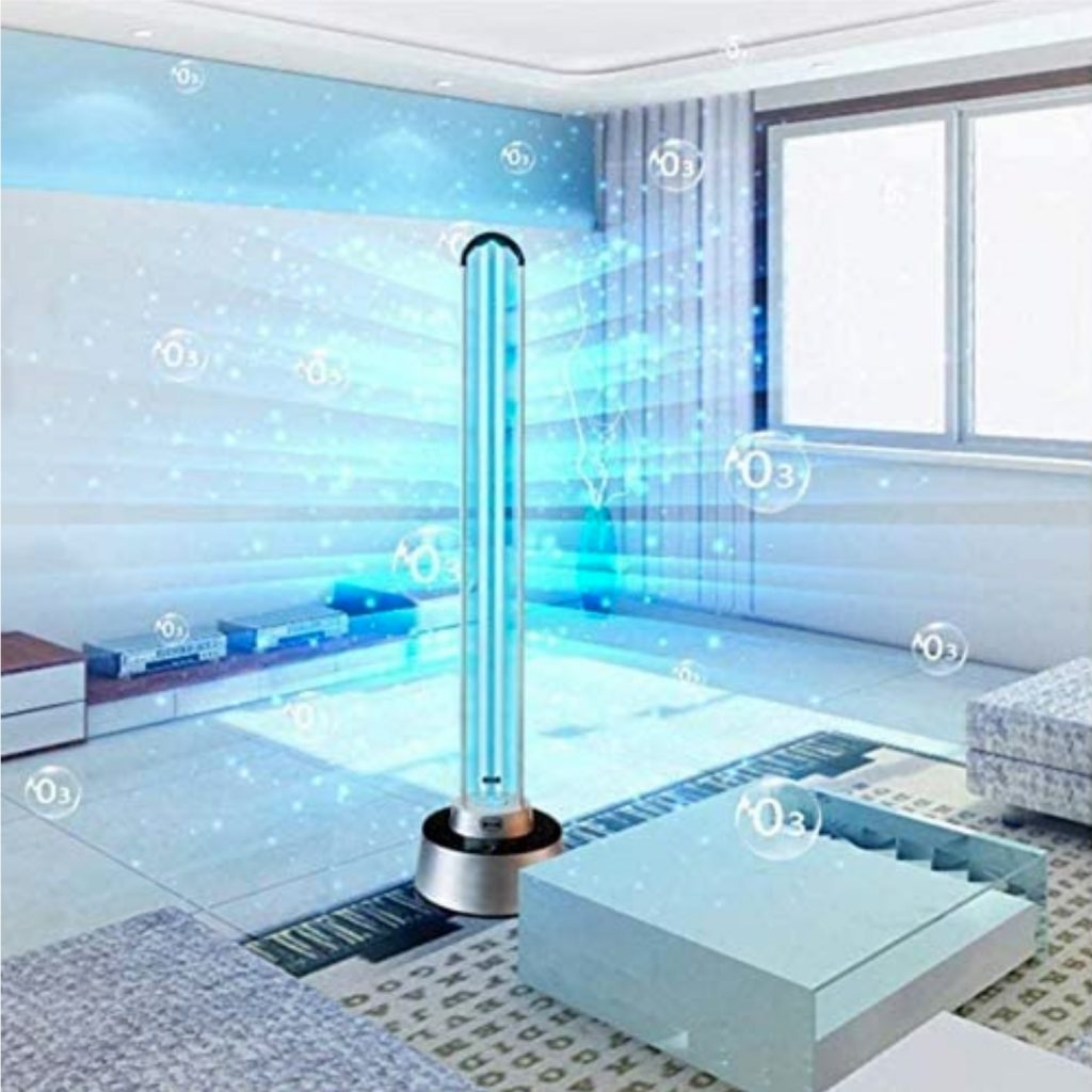
With no regulations to constrain them, manufacturers of high-power UV-C disinfection lamps are free to sell whatever they want to the unsuspecting consumer … and Amazon is assuredly there to help them. Enter “150 watt UV ozone” in the search bar for www.amazon.com and you will get over 140 results like this:
There are a number of reasons to be suspicious about the manufacturer’s claims for this product, but suppose we take the 150-watt electrical input power at face value. We can reasonably assume that the lamp ballast (remember that it is essentially a linear fluorescent lamp) has an efficiency of 90 percent. This means that 135 watts is being delivered to the mercury-vapor arc.
The radiant efficiency of a low-pressure mercury arc is about 45 percent, while the UV-C transmittance of fused quartz is about 90 percent, and so the lamp is emitting 55 watts of UV-C radiation.
The lamp itself, despite its outsized appearance in FIG. 4, is about 80 cm high. If we were to place a 60 cm diameter by 80 cm long tube over this lamp, it would have an inside surface area of roughly 15,000 cm2. The UV-C irradiance of this surface would therefore be 5.5 x 10⁷ microwatts divided by 1.5 x 10⁴ square centimeters, or about 3,650 μW/cm2 – over 6,000 times the ACGIH-recommended limit for 90 minutes’ exposure!
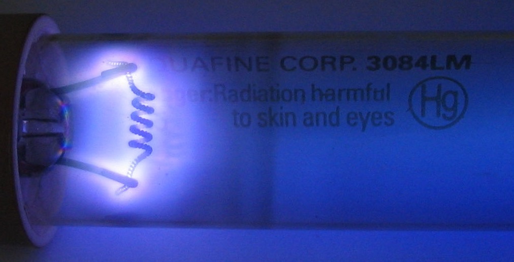
How can you tell whether the unit is activated? Ultraviolet radiation is by definition invisible, but someone sitting next to the unit in the dark, possibly watching television, may eventually notice a pretty violet glow around the lamp electrodes (Fig. 5). This will alert them that they will become mightily uncomfortable two to six hours later.
One reason to be suspicious about the manufacturer’s claims for this product is that it supposedly generates ozone. According to the manufacturer, “Ozone has sterilization and disinfection, in addition to formaldehyde and odor, ozone can fill the entire room without being affected by obstructions.”
Whatever the claim of formaldehyde refers to, ozone is a particularly toxic gas, even in minute concentrations of 0.1 parts per million (ppm). It smells like chlorine gas, and it can cause similar (and severe) damage to respiratory tissues. A low-pressure mercury arc emits both 254 nm and 185 nm UV-C radiation. The shorter wavelength radiation is capable of ionizing the molecular oxygen in the air surrounding the lamp and so create ozone, but the quartz or soft glass envelopes of UV disinfection lamps are doped such that they are opaque to 185 nm radiation. Some UV-C lamps do emit ozone, but they are only used for industrial applications such as municipal water disinfection (where it replaces chlorine).
Product safety information? The description for a similar product reads, “Do not look directly at the germicidal light source. Absorbing too much ultraviolet light can cause skin irritation and conjunctival damage.” This is regrettably what we get in the absence of enforced government regulations.
There are reasons to suspect some of the manufacturers’ descriptions of these products (many of which are identical apart from the manufacturer’s name), particularly when one manufacturer states that the product has an “ozone mode” and an “ozone-free mode,” where the latter is suitable for pregnant women and the elderly. How the doping of a quartz envelope designed to block 185 nm radiation from ionizing the surrounding air can be toggled on and off with the simple flip of a switch is left unexplained.
With over 140 products like these to choose from, the average consumer should feel … absolutely petrified.
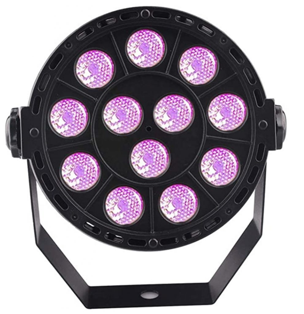
But rest assured! If you are concerned about your health, searching for “UV disinfection COVID” yields at least 20 UV sterilizer products that are available for purchase. One blatantly states, “Kill 99% COVID-19,” while another features a 10-watt battery-powered flashlight marketed as a “UVC Germicidal Lamp” with “Brightness: about 500 lumens.”
My favorite, however, must be the “UV COVID Indoor Sterilizer” shown in Figure 6. Lighting designers will understandably suspect that this is a theatrical LED luminaire, but the manufacturer assures us that it (somehow) emits “Ultraviolet wavelength of 253.7 nm.” Oh yes, and it can also be used for aromatherapy!
We are now living in different times, but one thing will always be the same: wherever there is a dire situation, there will be those among us willing and able to take advantage of our fears and gullibility. Say the words “ultraviolet disinfection” today and you will appreciate what technology has brought us – an online marketplace for charlatans and their wonderous pills that cure all ills.
UPDATE 20/04/23
For Europeans, the relevant standard concerning ultraviolet radiation in the workplace is Table 1.1 of EU-OSHA Directive 2006/25/EC, which specifies a maximum daily exposure to UV-C radiation of 30 J/m2, which is equivalent to the ACGIH recommendation of 3 mJ/cm2. The related publication “Non-binding Guide to Good Practice for Implementing Directive 2006/25/EC, Artificial Optical Radiation” (EC 2010) is highly recommended as an information source.
Worldwide, ISO 15858:2016, UV-C Devices – Safety Information – Permissible Human Exposure applies. This standard is applicable to in-duct UV-C systems, upper-air in room UV-C systems, portable in-room disinfection UV-C devices, and any other UV-C devices that may cause UV-C exposure to humans.
UPDATE 20/04/24
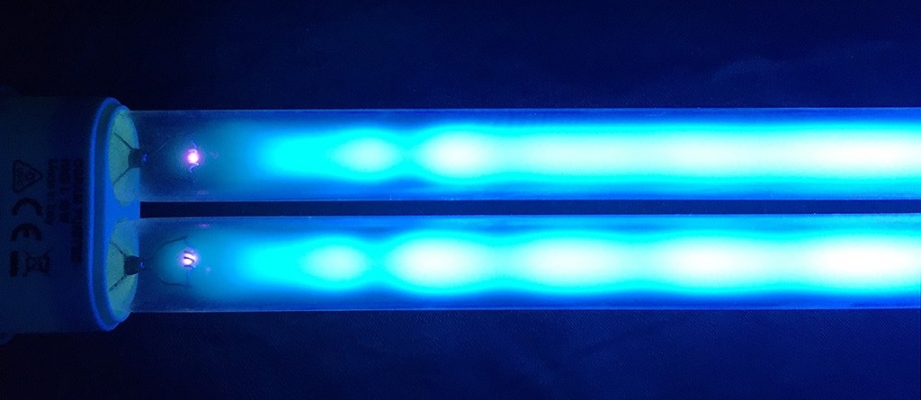
I am indebted to my colleague Dieter Lang of LEDVANCE for the following information and illustrations from his LinkedIn posting, “The Visible Spectrum of Mercury Low Pressure Lamps for Disinfection”:
FIG. 7 – Visible light image of UV-C germicidal lamp. (Source: Dieter Lang / LEDVANCE)
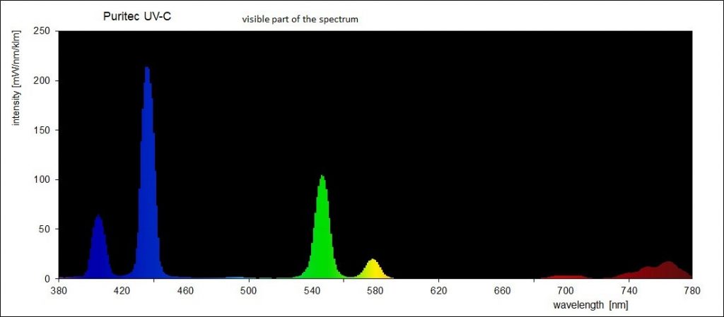
He also provided a useful and informative visible light spectrum for these lamps:
As Dieter writes, “The color shown in the photograph above is quite close to the real visual impression … of course you need to avoid looking at such a lamp without suitable eye protection.”
With this, I readily acknowledge that Figure 5 is somewhat misleading — it should be evident that high-power UV-C germicidal lamps are activated when viewed in a darkened room. Unfortunately, it was impossible to find photographs of such lamps in use that had not been doctored for advertising purposes (e.g., FIG. 4) by the manufacturer.
References
ACGIH. 2020. Ultraviolet Radiation: TLV(R) Physical Agents 7th Edition Documentation. Cincinnati, OH: American Conference of Governmental Industrial Hygienists.
Downes, A., and T. P. Blunt. 1877. “Researches on the Effect of Light Upon Bacteria and Other Organisms,” Proc. Royal Society of London 26:488-500.
EC. 2006. Directive 2006/25/EC – Artificial Optical Radiation. European Commission.
EC. 2010. Non-binding Guide to Good Practice for Implementing Directive 2006/25/EC, Artificial Optical Radiation.” European Commission.
Gates, F. L. 1931. “The Absorption of Ultraviolet Light by Bacteria,” J. General Physiology 14:31-42.
ISO. 2016. ISO 15858:2016, UV-C Devices – Safety Information – Permissible Human Exposure.
Trevisan, A., et al. 2006. “Unusual High Exposure to Ultraviolet-C Radiation,” Photochemistry and Photobiology 82:1077-1079.
SCHEER. 2017. Scientific Committee on Health, Environmental and Emerging Risks: Opinion on Biological Effects of UV-C Radiation Relevant to Health with Particular Reference to UV-C lamps, European Commission.
Wells, W. F., and M. G. Fair. 1935. “Viability of B. coli Exposed to Ultraviolet Radiation in Air,” Science 82:280-281.
Ian Ashdown, P. Eng, FIES, Senior Scientist, SunTracker Technologies Ltd.
Published: 19/11/14.
Whether you call it “circadian lighting,” “biologically effective lighting” or some other name, the principle is the same: the color and intensity of light can be used to regulate the timing of our biological clocks, or “circadian rhythms.” For architects and lighting designers, this is an opportunity to provide healthy and comfortable environments for building occupants.
From an academic perspective, circadian lighting represents the culmination of over two decades of research into the effects of light on circadian rhythms. While there remain a number of open questions and ongoing research to address them, it has been argued that we now know enough to translate this knowledge into practice with building code standards and recommended practices for architectural lighting design. From an engineering perspective … not so fast. A look at three metrics shows why.
WELL Building Standard
The WELL Building Standard v2 with Q1 Addenda is dedicated to the concept of building designs that promote healthy environments for living, working, learning and play. One of its hundreds of design guidelines is Feature 54, Circadian Lighting Design (https://standard. wellcertified.com/light/circadian-lighting-design).
The underlying concept is simple: predict or measure the Equivalent Melanopic Lux (EML) incident on the vertical plane at the eye level of the occupant. For work areas, the design requirements are then:
At 75% or more of workstations, provide at least 200 EML (including daylight if present) at four ft above the floor facing forward (to simulate the view of the occupant) between the hours of 9:00 am and 1:00 pm for every day of the year; or
For all workstations, provide maintained illuminance of at least 150 EML on the vertical plane facing forward.
There are similar requirements for living environments, breakrooms and learning areas. Unfortunately, architectural lighting design programs such as Lighting Analysts’ AGi32 and DIAL’s DIAL Evo do not predict EML. They do, however, predict photopic vertical illuminance, EV. All the designer has to do then is to calculate or measure EV values and multiply them by the melanopic ratio, R.
How do you calculate this ratio? These are the instructions from Table L2 of Feature 54: “To calculate the melanopic ratio of light, start by obtaining the light output of the lamp at each 5 nm increment, either from [the] manufacturer or by using a spectroradiometer. Then, multiply the output by the melanopic and visual curves given below to get the melanopic and visual responses. Finally, divide the total melanopic response by the total visual response and multiply the quotient by 1.218.”
The International WELL Building Institute helpfully provides a downloadable Excel spreadsheet to perform these calculations, which includes six sample spectra for common light sources—easy. Once again, from an engineering perspective, however … not so fast.
Questions, Questions …
Questions regarding the WELL Building Standard, or at least Feature 54, arise when considering how architectural lighting design is performed in practice. For example:
Unlike measurements of horizontal illuminance (EH), vertical illuminance (EV) measurements require both a specified position and a direction for the meter sensor. Four ft above the floor to “simulate the view of the occupant” makes sense, but it overlooks the reality that information on workstation locations and their associated furniture is often unavailable during the design phase.
Obtaining the spectral power distributions (SPDs) of luminaires from the manufacturer is in most cases all but impossible. This may change in the future as lighting design and analysis software programs become capable of utilizing this information directly, but for now it is mostly necessary to either manually digitize the manufacturers’ printed datasheets (if available) or measure representative products with a spectroradiometer. This is rarely practical during the design phase, when it is unlikely that specific products will have been identified.
Handheld spectroradiometers for field measurements are readily available, but they typically have a spectral resolution of 8 to 10 nm. They may report spectral power distributions in 5-nm or even 1-nm increments, but these are interpreted values. Depending on the light source (including particular fluorescent lamps and LED modules with “spiky” distributions), the calculation of equivalent melanopic lux from EV measurements may be insufficiently accurate. Following CIE recommendations for spectral metric calculations, a spectral resolution of at least 5 nm is required.
For workstations, what about the computer display monitors that the occupants will presumably be facing for most of the workday? With luminance values in the range of 250 to 350 candelas per sq meter, display monitors provide considerably more vertical illumination than the surrounding cubicle walls do, and they further have SPDs similar to white light LEDs of 6500K. If anything, they likely contribute more to the circadian lighting as perceived by the workstation occupants than the room lighting does. If they are to be considered, how should they be modeled? More important, what is their angular subtense in the occupant’s field of view? A dual 27-in. display fills much more of the occupant’s field of view than does a 17-in. display, for example.
Should daylight be included in the predictions or measurements of vertical illuminance? The amount of daylight entering an interior work space depends on the time and date, the building orientation and windows configuration, the sky condition (clear to overcast), the glazing transmittance, whether the blinds are open or closed, and the office partitions and furniture layout. Moreover, what is the SPD of the daylight on clear and overcast days? (The CCT of daylight can vary from 5500K for direct sunlight to more than 25000K for clear blue poleward sky.) Also, in modeling daylight, this should include the daylight diffusely reflected from the exterior ground, as it typically comprises some 10-20% of the daylight entering the space on overcast days.
How should multiple light sources, each with their own SPDs, be modeled? The occupant’s position and orientation at a “typical” workstation might include, depending on the time of day, direct sunlight, diffuse daylight, direct illumination from overhead luminaires, and indirect light from possibly strongly colored surfaces that are illuminated by both overhead luminaires and a desk lamp. It is all but impossible to predict the contributions of these light sources to the vertical illuminance, let alone calculate the resultant composite SPD as seen by the observer.
To put these questions into context, imagine the WELL design requirements being incorporated into Section 16500 clauses of a building specification contract document. It is one thing for an engineer or lighting designer to follow the WELL requirements as guidelines and feel comfortable in saying that the design is compliant; it is quite another when a contractual dispute arises or a building inspector decides to take in situ measurements. From a legal perspective, such ambiguities in the specifications are definitely not a good thing.
Circadian Stimulus
UL is currently preparing UL 24480, Recommended Practice and Design for Promoting Circadian Entrainment with Light for Day-Active People, a document that is based on the Circadian Stimulus (CS) metric developed by Rensselaer Polytechnic Institute’s Lighting Research Center. One of the key features of this document is that it relies on the user accessing the LRC’s CS Calculator (lrc.rpi.edu/cscalculator/), a web-based tool for converting predicted or measured vertical illuminance values into CS metric values.
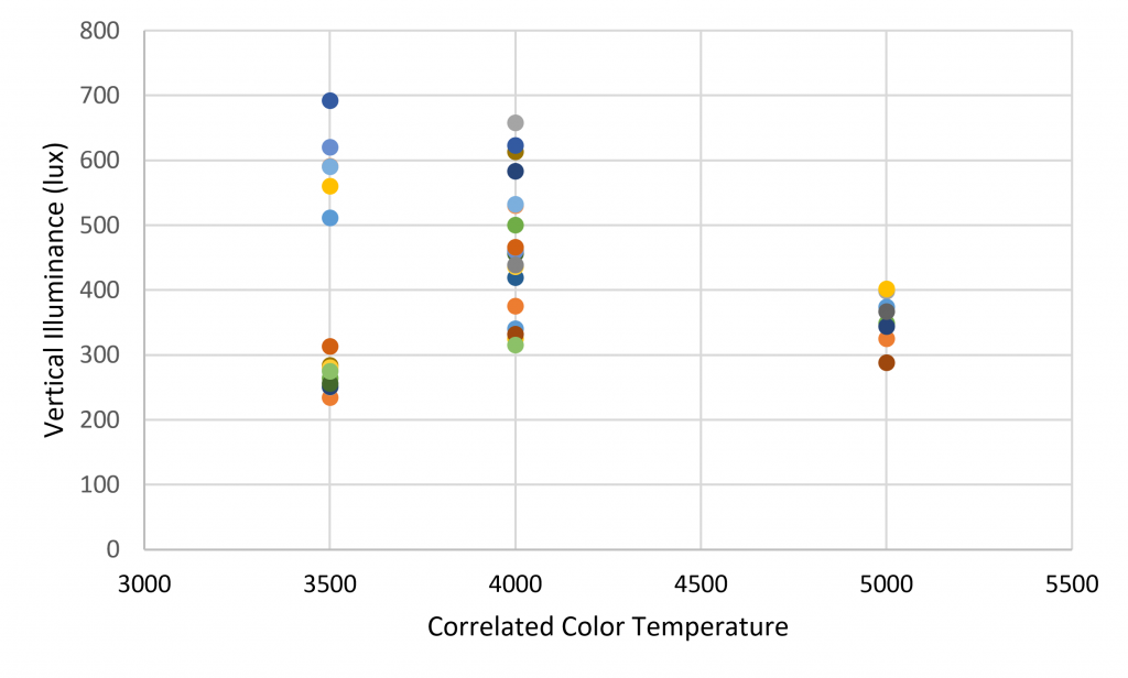
Unlike the WELL spreadsheet, the CS Calculator offers close to 200 different lamp SPDs for the designer to choose from. If, for example, you are interested in 3500K LED light sources, there are 19 SPDs to choose from, while for 4000K LEDs there are 20, and eight for 5000K … and therein lies a problem. For the designer, how do you choose?
Like the WELL’s EML metric, the CS metric is calculated from predicted or measured vertical illuminances, with minimum recommended CS values for different situations. If, for example, the design requires a CS value of 0.30, the designer chooses a light source from the list of options (or provides a custom SPD with 5-nm resolution); the calculator then determines the vertical illuminance needed to achieve this value.
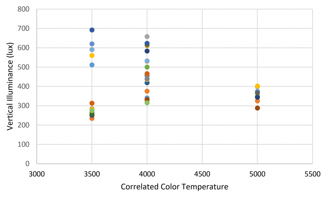
The problem is that even with the same correlated color temperature, the range of required vertical illuminances for the different LEDs is shocking (Figure 1). To be fair, some of these LED light sources are unconventional, including violet-pump LEDs (approximately 415 nm) with triphosphor coatings, and hybrid white-light LEDs combined with deep-red LEDs to boost the CRI R9 values. However, there is nothing to stop the designer from randomly choosing one of these products as a “typical” LED light source for calculation purposes.
3
SPDs to choose from, while for 4000-K LEDs there are twenty, and eight for 5000 K … and therein lies a
problem. For the designer, how do you choose?
Like the WELL’s EML metric, the CS metric is calculated from predicted or measured vertical
illuminances, with minimum recommended CS values for different situations. If, for example, the design
requires a CS value of 0.30, the designer chooses a light source from the list of options (or provides a
custom SPD with 5-nm resolution); the calculator then determines the vertical illuminance needed to
achieve this value.
The problem is that even with the same correlated color temperature, the range of required vertical
illuminances for the different LEDs is shocking (see Figure 1).
FIG. 1. Vertical illuminance required to achieve CS = 0.30 for different LED sources.
If nothing else, Figure 1 makes one point perfectly clear: there is no reasonable relationship between CCT and the CS metric, at least for 3500K and 4000K LEDs. The range of vertical illuminances for 3500K LEDs is 3:1, while that for 4000K LEDs is 2:1. Randomly choosing an LED product as representative of all LEDs with the same or similar CCT could lead to problematic consequences.
Compared to the 3500K and 4000K LEDs, the range of vertical illuminances for 5000K LEDs is quite small—only +/- 9%. The reason for this is that the eight LEDs appear to have almost identical SPDs above 500 nm, which is entirely due to the yellow-emitting phosphor blend. The only significant differences are the peak wavelengths of the blue-pump LEDs, which vary from 440 to 450 nm. This situation could, however, change with future developments in LED and phosphor technologies.
Additionally, what if the building specification permits “or equal” substitutions for luminaires? The CS metric value depends on the absolute spectral irradiance incident on the observer’s corneae, and so the luminaire product specification sheet would have to provide a graph of EV versus CS. Further, depending on the EV tolerance the designer is willing to accept, many more products may be disqualified compared to evaluation on luminous flux alone. As any experienced commercial electrical engineer will attest, this can lead to rather heated discussions between the engineering and architectural firms or with the electrical contractor.
Furthermore, the CS Calculator allows the designer to specify multiple light sources and combines their SPDs into a composite SPD as seen by the occupant. However, it is left as an exercise for the designer to calculate the relative contribution of each light source—including indirect light from possibly colored surfaces in the office space or wherever (and not to mention daylight with its range of possible CCTs)—to any predicted vertical illuminance. It is possible to do this with existing architectural lighting design programs, but only if the designer is willing to model and calculate the spatial light distribution in the environment separately for each type of light source. In addition, these programs do not take light source SPDs into account apart from their CCTs, so the results would be at best approximate.
EML versus CS
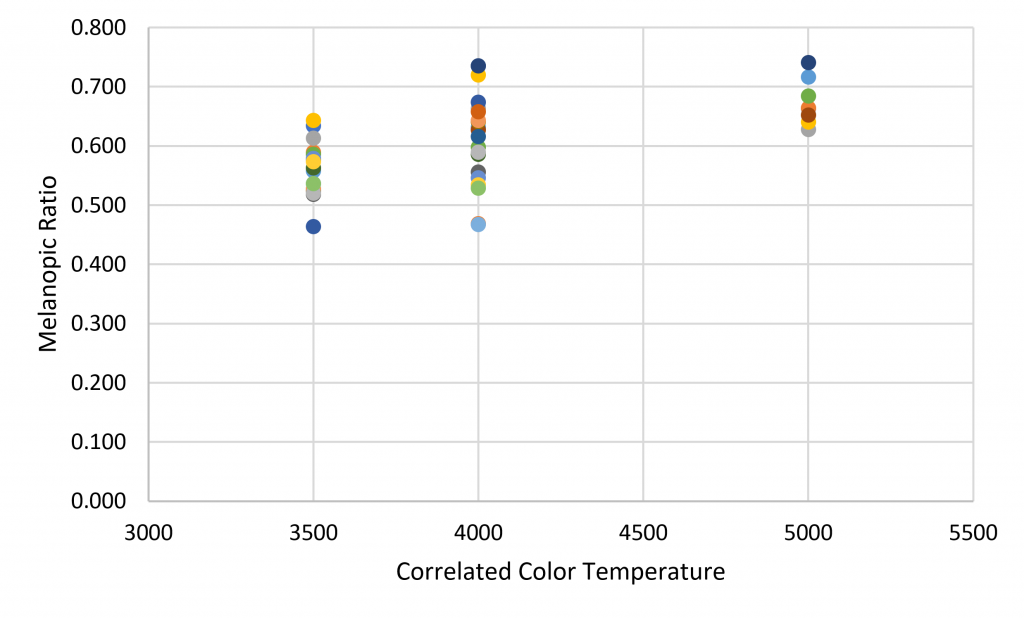
This is for the CS metric — what about the EML metric? Fortunately, the CS Calculator provides relative SPDs for each of its light sources, with resolution of 2 nm. Rescaling these SPDs to 5-nm resolution and using the WELL spreadsheet produces the melanopic ratios (R) shown in Figure 2.
FIG. 2. Melanopic ratio (R) for LEDs of 3500 K, 4000 K, and 5000 K.
There is still a 60% variation in the EML values for a given vertical illuminance value for LEDs of 4000K. This may be preferable (from an engineering perspective) to the 3:1 variation for the CS metric, but it is still an unreasonably wide range for lighting design purposes. It also begs the question: what are the criteria for choosing either the WELL or CS metrics apart from tolerances? Which circadian lighting metric better represents the effect of the lighting on circadian rhythm entrainment? Simply choosing the metric that offers the best results borders on unethical engineering practices.
In summary, we may now “know enough” about the effects of light on our circadian rhythms to design circadian lighting. Whether this is true is debatable, but it is also beside the point. From an engineering perspective, it is abundantly clear that we do not have the calculation tools needed to predict or measure circadian lighting metrics, including EML and CS, to acceptable engineering standards.
For reference, it is generally accepted that architectural lighting design software is capable of predicting horizontal and vertical illuminance values to within +/-10%, given reasonably accurate surface colors and reflectance values. With circadian lighting metrics, however, we are confounded by the variations between different LED products with the same CCT.
We are further confounded by what exactly it is we are expected to predict with our lighting design software or measure in the field. Simply saying “workstations” and “vertical illuminance” belies the complexity of both our architectural environments and our behaviors in them. This is not something that any standard or recommended practice can ever hope to reasonably address—there are simply too many variables for the designer to consider.
Regardless of what we
may know about the effects of circadian lighting on human health and wellbeing,
we may never be able to codify this knowledge in building design practices. It
is reasonable for standards organizations to offer design guidelines based on
what we know, and it is highly recommended that lighting designers learn the
principles and benefits of circadian lighting. These should not, however, be
codified as inflexible design requirements.
Ian Ashdown, P. Eng., FIES, Senior Scientist, SunTracker Technologies Ltd.
Published: 18/10/01.
Look at a greenhouse manufacturer’s product specifications and you will see that the light transmittance of single-pane clear glass is typically 88 to 91 percent. Compared to double-wall polycarbonate with a transmittance of 80 percent, it would seem that glass is the better choice. However, if you measure the photosynthetically active radiation (PAR) at the leaf canopy within the greenhouse, it is often only 40 to 60 percent of that measured outside the greenhouse. Why is this?
The answer is that these transmittance values were based on standard test procedures developed by the American Society of Testing Materials (ASTM), which require the incident light to be perpendicular to the glazing material. For greenhouses however, the incident light comes from direct sunlight, diffuse daylight, and daylight reflected from the ground and other exterior surfaces. In other words, light is incident upon the glazing material from all angles.
To better understand the issue, look at a sheet of clear glass. When it is perpendicular to your line of sight, it is essentially transparent. However, as you tilt the glass, you begin to notice reflections. These reflections increase in brightness until you are looking at the glass at a grazing angle, at which point it behaves essentially like a mirror.
This also happens, of course, with daylight entering the greenhouse. On a clear day, this is mostly direct sunlight, and so the amount of sunlight entering the greenhouse depends on the incidence angle θ (Fig. 1).
FIG. 1 – Incidence angle.
Assuming that the glazing material is perfectly transparent (that is, it does not absorb any light), the PAR light transmittance varies with the incidence angle as shown in FIG. 2.
FIG. 2 – Transmittance of direct sunlight through clear glazing.
To put this into perspective, consider a gutter-connected greenhouse with a 1:2 (30-degree) roof pitch and double-pane glass glazing that is located in Vancouver, Canada at a latitude of 49 degrees and oriented on an east-west axis. The solar elevation at noon on December 21st will be 18 degrees. The incidence angle will be 42 degrees, and so the transmittance of the south-facing roof panels will be 48 percent. We can now see where the “40 to 60 percent” figure come from.
It is important to note that these results apply only to clear glazing materials with smooth surfaces, such as glass and acrylic. For materials such as polyethylene and polycarbonate with rough or striated surfaces that tend to diffuse the incident light, it becomes more difficult to predict their optical characteristics. A better approach is to measure their transmittance for various incidence angles in a test laboratory.
Predicting the precise amount of daylight that will be incident upon the
leaf canopy in a greenhouse can be done, but it requires a horticultural
lighting design program that considers building latitude and orientation,
building layout and dimensions, glazing materials, date and time, weather
conditions, and more. For now, however, it is sufficient to see why the
measured light at the leaf canopy is considerably less than what is measured
outside.
This website uses cookies (mostly chocolate chip) to improve your experience. We'll assume you're ok with this, but you can opt-out if you wish. Cookie settingsACCEPT
Cookies Policy
Privacy Overview
This website uses cookies to improve your experience while you navigate through the website. Out of these cookies, the cookies that are categorized as necessary are stored on your browser as they are essential for the working of basic functionalities of the website. We also use third-party cookies that help us analyze and understand how you use this website. These cookies will be stored in your browser only with your consent. You also have the option to opt-out of these cookies. But opting out of some of these cookies may have an effect on your browsing experience.
Necessary cookies are absolutely essential for the website to function properly. This category only includes cookies that ensures basic functionalities and security features of the website. These cookies do not store any personal information.
Any cookies that may not be particularly necessary for the website to function and is used specifically to collect user personal data via analytics, ads, other embedded contents are termed as non-necessary cookies. It is mandatory to procure user consent prior to running these cookies on your website.