Ian Ashdown, P. Eng., FIES, Senior Scientist, SunTracker Technologies Ltd.
Published: 2015/07/22
UPDATE: Sports field lighting analysis added 15/10/12.
[An edited version of this article was published as “STREET LIGHTS: Light pollution depends on the light source CCT” in the October 2015 issue of LEDs Magazine.]
Most of you will be familiar with the International Dark-Sky Association (IDA), which was founded in 1988 to call attention to the problems of light pollution. It reminds us that light pollution threatens professional and amateur astronomy, disrupts nocturnal ecosystems, affects circadian rhythms of both humans and animals, and wastes over two billion dollars of electrical energy per year in the United States alone.
The IDA’s Fixture Seal of Approval program “provides objective, third-party certification for luminaires that minimize glare, reduce light trespass, and don’t pollute the night sky.” Recent changes to this program have reduced the maximum allowable correlated color temperature (CCT) from 4100K (neutral white) to 3000K (warm white). Previously-approved luminaires with CCTs greater than 3000K will have one year to comply with the new standard.
There are several reasons for this revised CCT limit. One reason is that many people prefer low-CCT outdoor lighting, especially in residential areas. As noted by Jim Benya in his LD+A article “Nights in Davis” (Benya 2015), the City of Davis was obliged to replace newly-installed 4800K street lighting with 2700K luminaires at a cost of $350,000 following residents’ complaints. As was noted in the article, “2700K LEDs are now only 10 percent less efficacious than 4000K,” so here was presumably minimal impact on the projected energy savings.
But another, arguably more important, reason is that high-CCT luminaires contribute more to light pollution on a per-lumen basis than do low-CCT luminaires. This is perhaps best demonstrated by the widely-disseminated graph presented in Luginbuhl et al. (2014) and shown in FIG. 1:
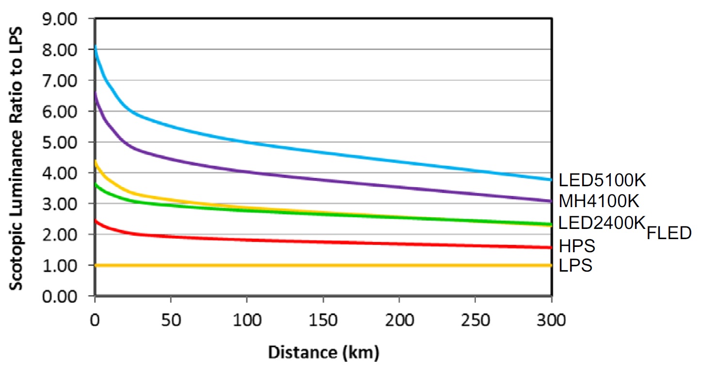
Luginbuhl et al. calculated this graph using a modified version of Garstang’s sky brightness model (Garstang 1986). What it shows is that the light pollution due to 5100K cool-white LED street lighting is approximately twice that of equivalent 2400K warm-white LED street lighting. According to the model, this relationship holds true regardless of the distance from the city to the remote astronomical observing site.
From the perspective of both professional and amateur astronomers as publicly represented by the International Dark-Sky Association, this graph is reason enough to require a maximum CCT of 3000K for the IDA’s Fixture Seal of Approval program.
There is however more to this story. While the graph shown in FIG. 1 may present clear evidence of the relationship between CCT and light pollution, we must remember that its data were calculated rather than measured. The question is whether it is reasonable to trust Garstang’s sky brightness model and its modification by Luginbuhl et al.
Garstang’s Model
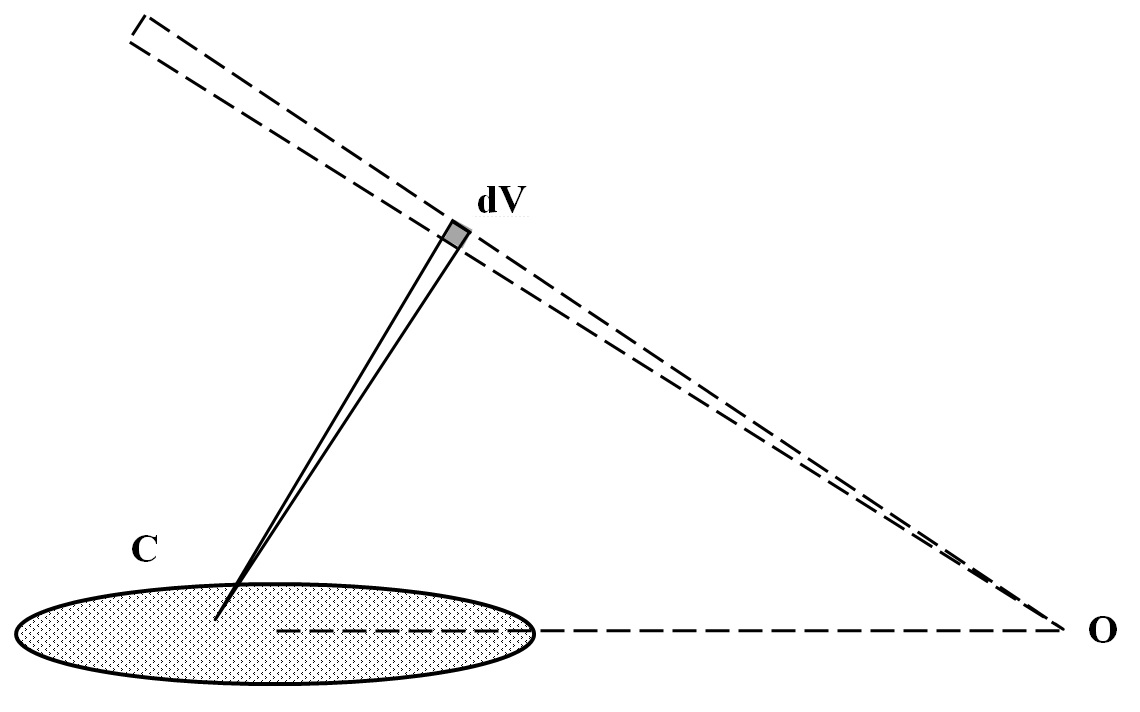
Garstang’s sky brightness model is conceptually simple. Referring to FIG. 2, imagine a city C and a distant observer O. The sky glow as seen by the observer is due to light emitted by the city streetlights that is scattered by the air molecules and aerosols in the atmosphere along the path of the observerís view direction. At any point along this path, the light will be scattered from the volume dV. The sky glow as seen by observer O is simply the sum of the scattered light for all such volumes along the path due to all of the luminaires within the city C.
Understanding the mathematics of Garstang’s model requires a reasonably good understanding of atmospheric optics (e.g., Liou 2002). This topic will not be discussed here beyond presenting (without explanation) Garstang’s equation for sky brightness b:
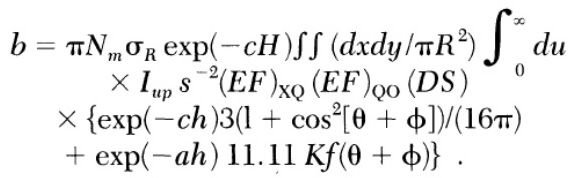
What is important for this discussion is that Garstang’s model assumes that the street lighting is monochromatic. He assumed a wavelength of 550 nm as being representative for visual astronomy.
We can have confidence that Garstang’s sky brightness model is reasonably accurate, based on recently-published validation studies by, for example, Duriscoe et al. 2013. With cities ranging from Flagstaff, AZ to Las Vegas, NV however, it is simply not possible to measure the influence of correlated color temperature on light pollution.
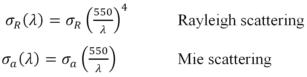
Wavelength Dependencies
Light pollution is due to both Rayleigh scattering from air molecules and Mie scattering from aerosols such as dust, smoke, and haze. Rayleigh scattering is strongly wavelength-dependent, with a probability proportional to λ-4 , where λ is the wavelength. The sky is blue because of Rayleigh scattering. Mie scattering is wavelength-independent, which is why the clear sky appears pale blue or white in heavily-polluted urban areas. (As an aside, the average distance a photon of blue light will travel through the atmosphere at sea level before undergoing Rayleigh scattering — its mean free path — is about 50 km. By comparison, the mean free path for a photon of red light is about 200 km.)
Luginbuhl et al. (2014) used these relationships to extend Garstang’s model for visible wavelengths between 400 nm and 700 nm in order to calculate FIG. 1:
While justifiable, this modification to Garstang’s model is somewhat ad hoc. In particular, the original model is a gross simplification of an exceedingly complex physical situation. While it has been validated in terms of sky brightness, this says nothing about whether Luginbuhl’s modifications result in similarly accurate solutions.
Radiative Flux Transfer
There have been more advanced light pollution models developed over the intervening thirty years, including Garstang 1991, Cinzano et al. 2000, Gillet et al. 2001, Aubé et al. 2005, Baddiley 2007, Kocifaj 2007, Luginbuhl et al. 2009, Kocifaj 2010, Kocifaj et al. 2010, Cizano and Falchi 2012, Kocifaj et al. 2014, Luginbuhl et al. 2014, and Aubé 2015.
Perhaps the most comprehensive light pollution model developed to date is Illumina, an open source program that was described in Aubé et al. 2005, and which is still under development. Unlike Garstang’s model (which was designed to execute on a 1980s-era Apple II computer), Illumina is a voxel-based radiative flux transfer program that can require weeks of computer time on a supercomputer with several thousand CPUs and terabytes of RAM (Aubé 2015).
The situation is similar to weather prediction models, where a simple model will give you a rough idea of what is going to happen, but it requires a supercomputer to perform massive amounts of data processing in order to have full confidence in the predictions. Simply put, Illumina models light pollution in a manner that would have been inconceivable thirty years ago.
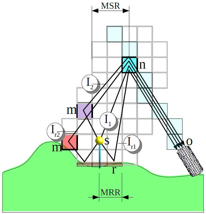
Unlike Garstang’s model, Illumina explicitly considers diffuse reflections from the ground and in-scattering of scattered light from volumes m into the volumes n visible to the observer. Garstang’s model includes an entirely ad hoc term for double scattering, but it is impossible to determine whether it correctly models the atmospheric optics.
The details of the program, however, are not as important for the purposes of this article as are the results recently reported by its author (Aubé 2015).
Modeling Sky Glow
What Aubé found with Illumina is that the combination of Rayleigh and Mie scattering results in a wavelength dependency described by λ-α , where α varies from 3.6 to 2.7 as the distance from the city center increases (FIG. 4).
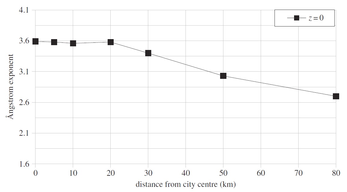
What FIG. 4 shows is that near the city center, Rayleigh scattering dominates. This is to be expected, as Rayleigh scattering is not directional — the light is scattered equally in all directions, including back down towards the observer.
FIG. 4 also shows that away from the city center, Mie scattering begins to dominate. This is also to be expected, as Mie scattering is directional — the light is preferentially scattered in the forward direction. It is therefore more likely to be scattered to a remote observer as it travels horizontally through the atmosphere.
Sky Glow versus CCT
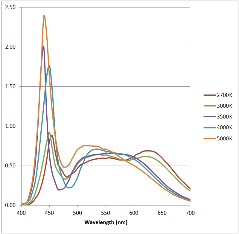
To apply Aubé’s results to the question of the influence of CCT on sky glow, we first need some representative white light LED spectral power distributions. The following normalized SPDs were digitized from Philips Lumileds’ Luxeon Rebel product catalog (FIG. 5):
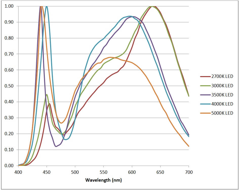
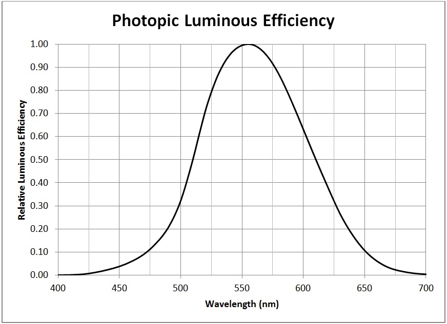
To provide a fair comparison, these SPDs need to be scaled such that the LEDs generate the same luminous intensity. To do this, we multiply the SPDs by the photopic luminous efficiency function at 5 nm intervals (FIG. 6):
and then sum the results to obtain the relative photopic intensities:
| CCT | Relative Luminous Intensity |
| 2700K | 0.88 |
| 3000K | 1.00 |
| 3500K | 1.12 |
| 4000K | 1.17 |
| 5000K | 0.94 |
Table 1
Dividing the normalized SPDs by these values gives:
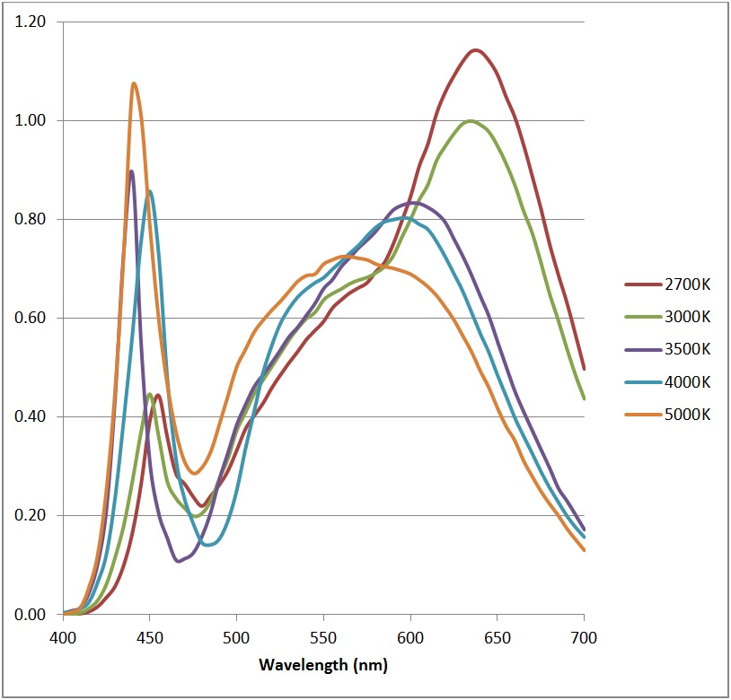
What FIG. 7 shows are the different spectral power distributions of the street lighting at city center for each CCT, assuming the same luminous flux output.
Now, using Aubé’s results and assuming an observing site 80 km (50 miles) from the city center, we multiply each 5 nm interval by (λ/550 nm)-2.7 to represent the wavelength dependency (FIG. 8):
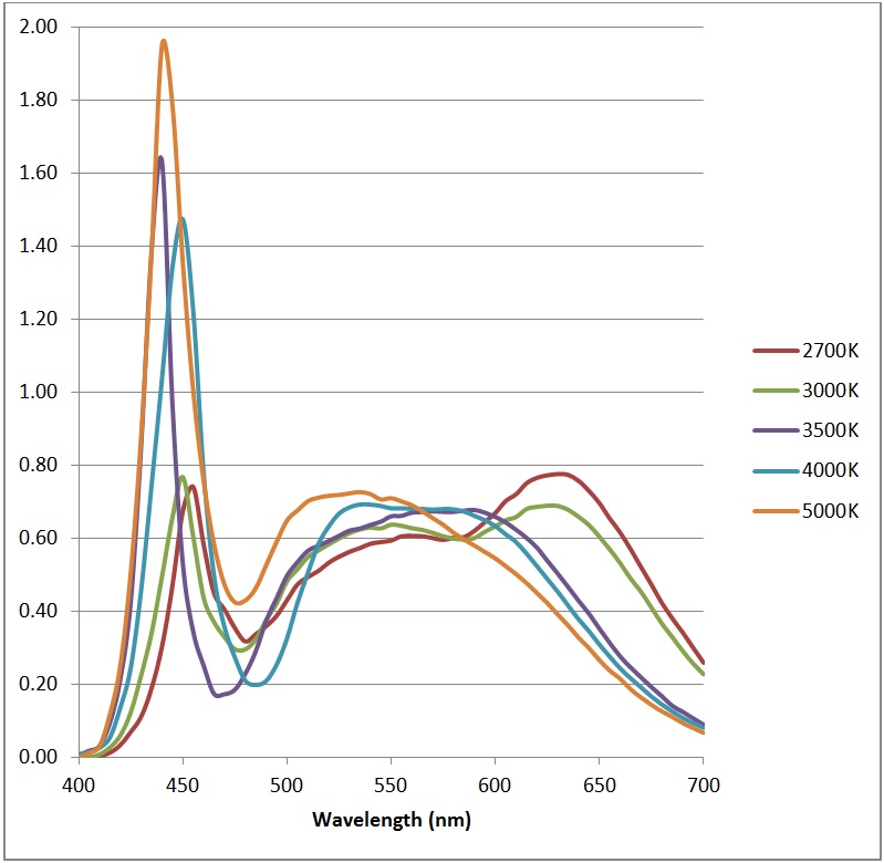
This is precisely what we might expect — blue light is preferentially scattered, bolstering our assumption that high-CCT lighting results in increased sky glow. (These SPDs represent the relative spectral radiance distribution at zenith from the observing site, which is perhaps the most useful definition of sky glow.)
If we assume scotopic (i.e., dark-adapted) visual observing conditions, we need to multiply these SPDs by the scotopic luminous efficiency function at 5 nm intervals (FIG. 9):
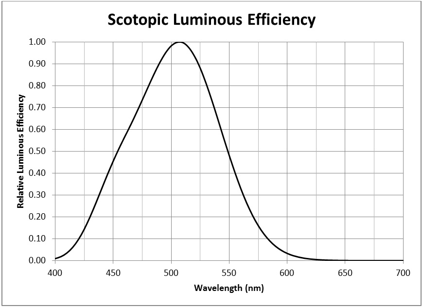
and sum the results to obtain the relative scotopic zenith luminance. The results are shown in Table 2:
| CCT | Relative Scotopic Luminance |
| 2700K | 0.96 |
| 3000K | 1.00 |
| 3500K | 1.04 |
| 4000K | 1.12 |
| 5000K | 1.42 |
Table 2 – Relative sky glow luminance at 80 km
This however is for a remote astronomical observing site, such as a dark-sky preserve. To understand what happens within the city center, we repeat the above procedure with α = 3.6 as per FIG. 4. Rayleigh scattering predominates, as shown by FIG. 10 with its greatly exaggerated blue peaks.
When we calculate the relative scotopic luminance of sky glow, however, we find almost identical results (Table 3).
| CCT | Relative Scotopic Luminance |
| 2700K | 0.96 |
| 3000K | 1.00 |
| 3500K | 1.05 |
| 4000K | 1.14 |
| 5000K | 1.45 |
Table 3 – Relative sky glow luminance at city center
This assumes, however, that the observer is completely dark-adapted. In an urban setting, the surrounding street lighting will most likely result in only partial dark adaptation, and so mesopic vision will apply. This means a blending of the photopic and scotopic luminous efficiency functions (FIG. 6 and FIG. 9). With the photopic function being much less sensitive to 450 nm blue light, the differences in relative sky glow luminance at city center will be (depending on the visual adaptation field of the observer) somewhere between that of Table 3 and Table 4, which assumes photopic adaptation:
| CCT | Relative Photopic Luminance |
| 2700K | 0.99 |
| 3000K | 1.00 |
| 3500K | 1.01 |
| 4000K | 1.02 |
| 5000K | 1.06 |
Table 4 – Relative sky glow luminance at city center (photopic adaptation)
Of course, with full photopic adaptation, the observer will not be able to see anything but the brightest stars and planets in the night sky, so it is best to rely on Table 3 for comparison purposes.
Given the above, the answer to our question is yes, it is reasonable to trust Garstangís sky brightness model and its modification by Luginbuhl et al. Aubé’s results, based on the much more comprehensive radiative flux transfer model used by Illumina, basically confirms the relationship between CCT and sky brightness as calculated by Luginbuhl et al. (2014).
Astronomical Considerations
According to Table 2, the increase in scotopic sky brightness for 4000K LEDs compared to 3000K LEDs is only 12 percent. Our perception of brightness, following Steven’s Power Law for extended light sources, means that we would see an increase in perceived sky brightness of only four percent! Surely this is not a reasonable justification for the IDA reducing the maximum allowable CCT from 4100K to 3000K for its Fixture Seal of Approval program?
Professional and amateur astrophotographers would vehemently disagree. Richard Wainscoat, Principal Investigator of the NASA-funded Pan-STARRS search for Near Earth Objects at the University of Hawaii, aptly called spectral power distributions of high-CCT LEDs such as that shown in FIG. 8 the “nightmare spectrum” (Betz 2015). Unfortunately, the peak 450 nm emission is right in the spectral region where natural airglow is low and there are important astronomical hydrogen and oxygen emission lines. Unlike the basically monochromatic emissions of low-pressure sodium lamps, it is impossible to filter out the blue LED emissions with band rejection filters. Limiting the CCT to 3000K reduces the contribution to light pollution in the blue region of the spectrum by a factor of two to three.
Allowing 4100K LEDs may be acceptable for casual stargazing, but not for astronomical research or astrophotography.
Ecological Considerations
According to the Fixture Seal of Approval requirements on the IDA Web site:
The case against blue light is well founded with regard to discomfort glare, circadian rhythm disruption, light scattering, sky glow, and biological system disruption in wildlife.
Outdoor lighting with high blue light content is more likely to contribute to light pollution because it has a significantly larger geographic reach than lighting with less blue light. In natural settings, blue light at night has been shown to adversely affect wildlife behavior and reproduction. This is true even in cities, which are often stopover points for migratory species.
The comment about cities is particularly germane in view of FIG. 10, where the light pollution in the blue region of the spectrum from 5000K LEDs is nearly three times that from 3000K LEDs. (To be fair however, this applies to clear skies only. For cloudy skies, Mie scattering from the water droplets dominates, and so the spectral power distribution of the reflected street lighting is essentially that of the lighting itself. On the other hand, much more light is reflected back towards the ground, greatly increasing light pollution.)
Summary
The purpose of this article was to examine the International Dark-Sky Association’s requirement of LEDs with CCTs of 3000K or less for their Fixture Seal of Approval program. Using recent research results based on a comprehensive light pollution model (Aubé 2015), it was found that the concerns over high-CCT LEDS are well-founded. While 4000K LEDs may be acceptable for casual star-gazing, they are anathema for astronomers and wildlife.
In short, requiring LED street lighting with CCTs of 3000K or less is completely justifiable.
UPDATE 2015/10/12
The analysis presented above assumes a gray world with spectrally neutral reflectance. This is a reasonable assumption in that most roadway surfaces — concrete and asphalt — are not strongly colored. In other words, the light reflected from the ground will have approximately the same spectral power distribution as the incident light.
Suppose, however, that we have an outdoor sports arena with a grass field. The spectral reflectance distribution for Kentucky bluegrass (Poa pratensis) is shown in FIG. 11. The pronounced green peak is expected, given the grass-green color. What is more interesting, however, is the relatively low reflectance in the blue region of the visible spectrum.

If we multiply the typical LED spectral power distributions shown in FIG. 7 with the grass spectral reflectance distribution on a per-wavelength basis, the overhead sky glow spectral power distribution at 50 km from the city center becomes that shown in FIG. 12. The blue peaks are still present, but they have been reduced by a factor of four relative to the remainder of the spectral power distribution.

The number of outdoor sports arenas may be relatively small, but they generate a surprising amount of light when they are illuminated at night. Using data from the U.S. Department of Energyís 2010 U.S. Lighting Market Characterization report (DOE 2012), it can be estimated (with reasonable assumptions for typical lamp lumens) that the distribution of outdoor lighting in the United States is:
| Outdoor Lighting | Percent Lumens |
| Roadway | 48.2 |
| Parking | 34.0 |
| Building Exterior | 10.2 |
| Stadium | 6.0 |
| Billboard | 0.8 |
| Traffic Signals | 0.7 |
| Airfield | 0.1 |
| Railway | 0.0 |
Table 5 – Light pollution sources (approximate)
This is, of course, a global view — light pollution next to a large outdoor sports arena can be a significant concern for residential neighborhoods. The best that can be done is shield the luminaires appropriately, and to turn on the sports field lighting only when it is needed.
In terms of correlated color temperature, the Federation Internationale de Football Association (FIFA) specifies a minimum CCT of 4000K for football stadiums (FIFA 2007), while the National Football League (NFL) requires a CCT of 5600K (Lewis and Brill 2013). These are arguably acceptable in that green grass fields greatly alleviate the “nightmare spectrum” problem.
(Thanks to Brad Schlesselman of Musco Lighting for providing the grass spectral reflectance distribution and thereby inspiring this analysis.)
References
Aubé, M., L. Franchomme-Fosse, P. Robert-Staehler, and V. Houle. 2005. “Light Pollution Modelling and Detection in a Heterogeneous Environment: Toward a Night Time Aerosol Optical Depth Retrieval Method,” Proc. SPIE Volume 5890.
Aubé, M. 2015. “Physical Behaviour of Anthropogenic Light Propagation into the Nocturnal Environment,” Philosophical Transactions of the Royal Society B 370(1667):20140117.
Baddiley, C. 2007. “A Model to Show the Differences in Skyglow from Types of Luminaire Designs,” Starlight 2007. La Palma, Canary Islands.
Benya, J. R. 2015. “Nights in Davis,” LD+A 45(6):32-34.
Betz, E. 2015. “A New Fight for the Night,” Astronomy 43(6):46-51.
Cinzano, P., and F. J. D. Castro. 2000. “The Artificial Sky Luminance and the Emission Angles of the Upward Light Flux,” Journal of the Italian Astronomical Society 71(1):251.
Cinzano, P., and F. Falchi. 2012. “The Propagation of Light Pollution in the Atmosphere,” Monthly Notices of the Royal Astronomical Society 427(4):3337-3357.
DOE. 2012. 2010 U.S. Lighting Market Characterization. U.S. Department of Energy Building Technologies Program.
Duriscoe, D. M., C. B. Luginbuhl, and C. D. Elvidge. 2013. “The Relation of Outdoor Lighting Characteristics to Sky Glow from Distant Cities,” Lighting Research and Technology 46(1):35-49.
FIFA. 2007. Football Stadiums: Technical Recommendations and Requirements, 4th Edition. Zurich, Switzerland: Federation Internationale de Football Association.
Garstang, R. H. 1986. “Model for Artificial Night-Sky Illumination,” Publications of the Astronomical Society of the Pacific 98:364-375.
Garstang, R. H. 1991. “Dust and Light Pollution”, Publications of the Astronomical Society of the Pacific 103:1109-1116.
Gillet, M., and P. Rombauts. 2001. “Precise Evaluation of Upward Flux from Outdoor Lighting Installations (Applied in the Case of Roadway Lighting),” Proc. International Conference on Light Pollution. Serena, Chile.
Kocifaj, M. 2007. “Light-Pollution Model for Cloudy and Cloudless Night Skies with Ground-Based Light Sources,” Applied Optics 46(15):3013-3022.
Kocifaj, M. 2010. “Modelling the Spectral Behaviour of Night Skylight Close to Artificial Light Sources,” Monthly Notices of the Royal Astronomical Society 403:2105-2110.
Kocifaj, M., M. Aubé, and I. Kohút. 2010. “The Effect of Spatial and Spectral Heterogeneity of Ground-Based Light Sources on Night-Sky Radiances,” Monthly Notices of the Royal Astronomical Society 409:1203-1212.
Kocifaj, M., and S. Lamphar. 2014. “Skyglow: A Retrieval of the Approximate Radiant Intensity Function of Ground-Based Light Sources,” Monthly Notices of the Royal Astronomical Society 443:3405-3413.
Lewis, D., and S. Brill. 2013. Broadcast Lighting: NFL Stadium Lighting. The Design Lighting Group Inc.
Liou, K. N. 2002. An Introduction to Atmospheric Radiation, Second Edition. New York, NY: Academic Press.
Luginguhl, C. B., D. M. Duriscoe, C. W. Moore, A. Richman, G. W. Lockwood, and D. R. Davis. 2009. “From the Ground Up II: Sky Glow and Near-Ground Artificial Light Propagation in Flagstaff, Arizona.” Publications of the Astronomical Society of the Pacific 121 (876):204-212.
Luginbuhl, C. B., P. A. Boley, and D. R. Davis. 2014. “The Impact of Light Source Spectral Power Distribution on Sky Glow,” Journal of Quantitative Spectroscopy & Radiative Transfer 139:21-26.